Duane’s reliability growth (1964)

James Duane, at General Electric’s Motor and Generator Department, plotted the failure records of five development programmes, from hydraulic devices to aircraft generators. On log-log paper the cumulative MTBF, total test time over total failures, rose along a straight line, each programme with a slope near 0.5. A straight line is a power law, \(\theta_c = K t^\alpha\) (reliability_growth_duane()), so a few months of data predict how much more testing a reliability target needs. Because the failure count is \(N(t) = t^{1-\alpha}/K\), the current failure rate is \(dN/dt\), and the instantaneous MTBF is the cumulative one divided by \(1 - \alpha\).

import matplotlib.pyplot as plt
import numpy as np

from engineeringkit.reliability import reliability_growth_duane

A simulated test-fix-test programme

Failure times follow the power-law process \(N(t) = t^{1-\alpha}/K\) (Crow’s AMSAA model): a unit-rate Poisson process mapped through the inverse of \(N\). Time unit: hours.

K_true, alpha_true = 2.0, 0.45
rng = np.random.default_rng(1964)
arrivals = np.cumsum(rng.exponential(size=150))
failure_times = (K_true * arrivals) ** (1 / (1 - alpha_true))
cumulative_mtbf = failure_times / np.arange(1, failure_times.size + 1)

# Duane's straight line through the log-log points.
slope, intercept = np.polyfit(np.log(failure_times), np.log(cumulative_mtbf), 1)
K_fit = np.exp(intercept)
print(f"fitted alpha = {slope:.3f} (true {alpha_true}), K = {K_fit:.2f} h^(1-alpha) (true {K_true})")
print(f"{failure_times.size} failures in {failure_times[-1]:.0f} h of testing")

fitted alpha = 0.443 (true 0.45), K = 2.09 h^(1-alpha) (true 2.0)
150 failures in 34847 h of testing

Cumulative and instantaneous MTBF

The current MTBF is the reciprocal of the slope of the failure count, which the simulation gives directly as a finite difference.

t = np.geomspace(failure_times[0], failure_times[-1], 200)
theta_c = reliability_growth_duane(t, K_fit, slope)
theta_i = theta_c / (1 - slope)
count = t ** (1 - slope) / K_fit
numeric_instantaneous = 1 / np.gradient(count, t)
assert np.allclose(numeric_instantaneous[5:-5], theta_i[5:-5], rtol=1e-3)

target = 400.0
t_needed = ((1 - slope) * target / K_fit) ** (1 / slope)
print(f"instantaneous MTBF now: {theta_i[-1]:.0f} h; {target:.0f} h is reached after {t_needed:.0f} h of testing")

fig, ax = plt.subplots(figsize=(7, 4.2))
ax.loglog(failure_times, cumulative_mtbf, "o", ms=3, color="0.5", label="cumulative MTBF of the test data")
ax.loglog(t, theta_c, "C0", label=rf"Duane fit $K t^{{\alpha}}$, $\alpha$ = {slope:.2f}")
ax.loglog(t, theta_i, "C3", label=r"instantaneous MTBF $\theta_c/(1-\alpha)$")
ax.axhline(target, color="k", ls=":", lw=1)
ax.set(xlabel="cumulative test time [h]", ylabel="MTBF [h]", ylim=(1, 1000), title="Reliability growth on log-log paper")
ax.legend()
fig.tight_layout()

assert abs(slope - alpha_true) < 0.05
assert np.isclose(float(reliability_growth_duane(t_needed, K_fit, slope)) / (1 - slope), target)

plt.show()

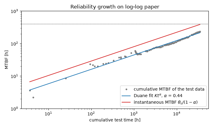
instantaneous MTBF now: 386 h; 400 h is reached after 37872 h of testing