Haar’s wavelet (1910)

In his 1909 dissertation, published in 1910, Alfréd Haar built an orthonormal basis from a single step function: the difference between the two halves of an interval, shrunk and shifted to every scale and position (haar_transform()). It was the first wavelet, though the word came 70 years later. Each Haar function lives on a short interval, so a jump in a signal touches only a few coefficients at each scale. A sine, by contrast, extends over all time and smears a jump over every coefficient. The transform keeps the signal’s energy and is inverted exactly (inverse_haar_transform()).

import matplotlib.pyplot as plt
import numpy as np

from engineeringkit.signal_processing import dft, energy, haar_transform, inverse_haar_transform

A piecewise signal with jumps

n = 1024
t = np.arange(n) / n
x = np.where(t < 0.3, 1.0, np.where(t < 0.55, -0.5, 0.8)) + 0.3 * np.sin(2 * np.pi * 2 * t)
coefficients = haar_transform(x)
print(f"{len(coefficients) - 1} levels; detail lengths {[c.size for c in coefficients[1:]]}")
assert np.isclose(sum(energy(c) for c in coefficients), energy(x))
assert np.allclose(inverse_haar_transform(coefficients), x)

10 levels; detail lengths [1, 2, 4, 8, 16, 32, 64, 128, 256, 512]

Keep the largest 5% of coefficients

Zero every Haar coefficient but the largest 51, and do the same with the Fourier coefficients. The Haar approximation keeps the jumps sharp; the Fourier one rings around them (Gibbs’s phenomenon).

keep = n // 20
flat = np.concatenate(coefficients)
threshold = np.sort(abs(flat))[-keep]
sizes = np.cumsum([c.size for c in coefficients])[:-1]
compressed = inverse_haar_transform(np.split(np.where(abs(flat) >= threshold, flat, 0.0), sizes))

X = dft(x)
fourier_threshold = np.sort(abs(X))[-keep]
fourier = np.fft.ifft(np.where(abs(X) >= fourier_threshold, X, 0)).real

errors = {"Haar": np.sqrt(np.mean((compressed - x) ** 2)), "Fourier": np.sqrt(np.mean((fourier - x) ** 2))}
for name, error in errors.items():
    print(f"{name:7s}: RMS error keeping {keep} of {n} coefficients = {error:.4f}")
assert errors["Haar"] < errors["Fourier"]

fig, axes = plt.subplots(1, 2, figsize=(10, 3.8))
axes[0].plot(t, x, "k", lw=2, label="signal")
axes[0].plot(t, compressed, label=f"Haar, {keep} coefficients")
axes[0].plot(t, fourier, lw=0.8, label=f"Fourier, {keep} coefficients")
axes[0].set(xlabel="t", xlim=(0.2, 0.65))
axes[0].legend(fontsize=8)

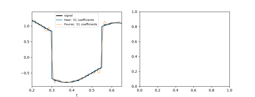
Haar   : RMS error keeping 51 of 1024 coefficients = 0.0144
Fourier: RMS error keeping 51 of 1024 coefficients = 0.0790

<matplotlib.legend.Legend object at 0x11110a710>

Where the energy sits

The large detail coefficients cluster at the jumps, at every scale.

for level, detail in enumerate(coefficients[1:][::-1], start=1):
    positions = (np.arange(detail.size) + 0.5) / detail.size
    axes[1].plot(positions, np.full(detail.size, level), "|", color="0.85")
    big = abs(detail) > 0.05
    axes[1].plot(positions[big], np.full(big.sum(), level), "|", color="C3", ms=12)
for jump in (0.3, 0.55):
    axes[1].axvline(jump, color="k", lw=0.5)
axes[1].set(xlabel="position", ylabel="level (1 = finest)", title="Detail coefficients above 0.05")
fig.tight_layout()

finest = coefficients[-1]
big_positions = (np.flatnonzero(abs(finest) > 0.05) + 0.5) / finest.size
assert np.all(np.min(abs(big_positions[:, None] - np.array([0.3, 0.55])), axis=1) < 0.01)

plt.show()