Navier’s beam theory (1826)

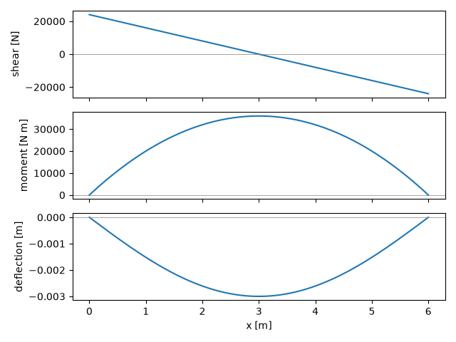
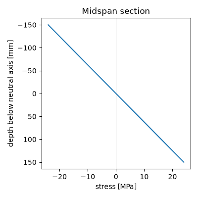
Navier’s 1826 lectures at the École des ponts et chaussées put beam theory in its modern form: plane sections stay plane, the neutral axis passes through the centroid, the stress is \(\sigma = My/I\) (bending_stress()) and the curvature is \(y'' = M/(EI)\). The example loads a steel beam (SimplySupportedBeam), checks the midspan deflection \(5wL^4/(384EI)\), and checks that the stress profile carries no net force and exactly the applied moment.

import matplotlib.pyplot as plt
import numpy as np
from scipy.integrate import simpson

from engineeringkit.structural_engineering import SimplySupportedBeam, bending_stress, rectangular_second_moment

Shear, moment and deflection

L, E, w = 6.0, 200e9, 8e3
b, h = 0.10, 0.30
I = rectangular_second_moment(b, h)
result = SimplySupportedBeam(L, E, I).solve_uniform_load(w, n=601)
summary = result.summary()
print(f"max moment {summary['max_abs_moment'] / 1e3:.1f} kN m, midspan deflection {1e3 * summary['max_abs_deflection']:.2f} mm")
assert np.isclose(summary["max_abs_moment"], w * L**2 / 8)
assert np.isclose(summary["max_abs_deflection"], 5 * w * L**4 / (384 * E * I))

fig, axes = result.plot()
for ax, label in zip(axes, ["shear [N]", "moment [N m]", "deflection [m]"]):
    ax.set_ylabel(label)
fig.tight_layout()

max moment 36.0 kN m, midspan deflection 3.00 mm

The stress across the midspan section

With y measured downward, a sagging moment puts the bottom in tension.

M = summary["max_abs_moment"]
y = np.linspace(-h / 2, h / 2, 401)
sigma = bending_stress(M, y, I)
net_force = simpson(sigma * b, x=y)
resisting_moment = simpson(sigma * b * y, x=y)
print(f"peak stress {sigma.max() / 1e6:.1f} MPa, net force {net_force:.2e} N, moment {resisting_moment / 1e3:.1f} kN m")
assert abs(net_force) < 1e-6 * M / h
assert np.isclose(resisting_moment, M)

fig, ax = plt.subplots(figsize=(4, 4))
ax.plot(sigma / 1e6, y * 1e3)
ax.axvline(0, color="gray", lw=0.5)
ax.invert_yaxis()
ax.set(xlabel="stress [MPa]", ylabel="depth below neutral axis [mm]", title="Midspan section")
fig.tight_layout()

plt.show()

peak stress 24.0 MPa, net force 0.00e+00 N, moment 36.0 kN m