Hess’s law and the heat of combustion (1840)

Germain Henri Hess, a chemist in St Petersburg, measured the heat released by reactions carried out in different steps. In 1840 he found that the total heat depends only on the initial and final states, not on the route. A heat of reaction is then the difference between the enthalpies of formation of the products and of the reactants. Combined with Lavoisier’s conservation of mass (combustion_products(), stoichiometric_air_fuel_ratio()), that gives a fuel’s heating value (heating_value()). Burning the fuel adiabatically with NIST’s product enthalpies gives the flame temperature (adiabatic_flame_temperature()).

import matplotlib.pyplot as plt
import numpy as np

from engineeringkit.thermodynamics import (
    adiabatic_flame_temperature,
    combustion_products,
    heating_value,
    stoichiometric_air_fuel_ratio,
)

Heating values from enthalpies of formation

Standard enthalpies of formation at 25 °C [J/mol]: methane gas -74.87 kJ, propane gas -103.85 kJ, liquid octane -249.95 kJ. The higher heating value condenses the product water; the lower leaves it as vapour.

fuels = {"methane": (1, 4, -74.87e3), "propane": (3, 8, -103.85e3), "octane (l)": (8, 18, -249.95e3)}
for name, (c, h, h_f) in fuels.items():
    lhv, hhv = heating_value(c, h, h_f_fuel=h_f), heating_value(c, h, h_f_fuel=h_f, water="liquid")
    afr = stoichiometric_air_fuel_ratio(c, h)
    print(f"{name}: LHV {lhv / 1e6:.1f} MJ/kg, HHV {hhv / 1e6:.1f} MJ/kg, stoichiometric air-fuel ratio {afr:.1f}")
assert np.isclose(heating_value(1, 4, h_f_fuel=-74.87e3), 50.0e6, rtol=0.002)  # the tabulated LHV of methane

methane: LHV 50.0 MJ/kg, HHV 55.5 MJ/kg, stoichiometric air-fuel ratio 17.2
propane: LHV 46.4 MJ/kg, HHV 50.3 MJ/kg, stoichiometric air-fuel ratio 15.6
octane (l): LHV 44.4 MJ/kg, HHV 47.9 MJ/kg, stoichiometric air-fuel ratio 15.1

The adiabatic flame temperature

With no heat lost, all the heat of reaction warms the products. Excess air dilutes the flame; preheating the air raises it. Real flames above about 2000 K are cooler because CO2 and H2O dissociate, which this model ignores.

excess = np.linspace(0, 3, 31)
fig, ax = plt.subplots(figsize=(6, 3.5))
for T_air in (298.15, 600.0):
    temps = [adiabatic_flame_temperature(1, 4, h_f_fuel=-74.87e3, excess_air=e, T_air=T_air) for e in excess]
    ax.plot(100 * (1 + excess), temps, label=f"air at {T_air - 273.15:.0f} °C")
ax.set(xlabel="theoretical air [%]", ylabel="adiabatic flame temperature [K]", title="Methane in air, complete combustion")
ax.legend()
fig.tight_layout()

T_stoich = adiabatic_flame_temperature(1, 4, h_f_fuel=-74.87e3)
products = ", ".join(f"{n:.2f} {k}" for k, n in combustion_products(1, 4).items())
print(f"methane, stoichiometric: {T_stoich:.0f} K; products per mol of fuel: {products}")
T_octane = adiabatic_flame_temperature(8, 18, h_f_fuel=-249.95e3, excess_air=3.0)
print(f"liquid octane with 400% theoretical air: {T_octane:.0f} K (Çengel and Boles: 962 K)")
assert 2300 < T_stoich < 2350 and abs(T_octane - 962) < 3

plt.show()

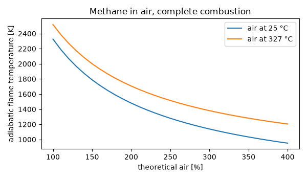
methane, stoichiometric: 2327 K; products per mol of fuel: 1.00 CO2, 2.00 H2O, 0.00 O2, 7.52 N2
liquid octane with 400% theoretical air: 962 K (Çengel and Boles: 962 K)