Rankine’s cycle with reheat and feedwater heating (1859)

Rankine’s pump, boiler, engine and condenser became the modern power station by three changes that raise the mean temperature at which heat is added. Superheating heats the steam beyond saturation. Reheating returns it to the boiler halfway through the expansion. Feedwater heating preheats the boiler water with steam bled from the turbine. Each also keeps the turbine exhaust dry. rankine_cycle() analyses the plant state by state with IAPWS-IF97. The example reproduces Çengel and Boles’s three textbook plants at 15 MPa, 600 °C and 10 kPa.

import matplotlib.pyplot as plt
import numpy as np

from engineeringkit.thermodynamics import carnot_efficiency, rankine_cycle, saturation_temperature

Simple, reheat and regenerative plants

plants = {
    "simple": rankine_cycle(15e6, 10e3, 873.15),
    "reheat at 4 MPa": rankine_cycle(15e6, 10e3, 873.15, reheat_pressure=4e6, T_reheat=873.15),
    "open heater at 1.2 MPa": rankine_cycle(15e6, 10e3, 873.15, feedwater_pressure=1.2e6),
    "both": rankine_cycle(15e6, 10e3, 873.15, reheat_pressure=4e6, T_reheat=873.15, feedwater_pressure=1.2e6),
}
for name, res in plants.items():
    s = res.summary()
    quality, bleed = s["turbine_exit_quality"], s["bleed_fraction"]
    print(f"{name:24s} η = {s['efficiency']:.3f}, exit quality {quality:.3f}, bleed {bleed:.3f}, net {s['net_work'] / 1e3:.0f} kJ/kg")
# Çengel and Boles, Examples 10-3, 10-4 and 10-5: 43.0%, 45.0% and 46.3%
assert [round(plants[k].efficiency, 3) for k in ("simple", "reheat at 4 MPa", "open heater at 1.2 MPa")] == [0.430, 0.450, 0.463]

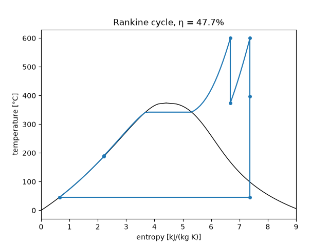
fig, ax = plants["both"].plot()
ax.set(xlim=(0, 9))

simple                   η = 0.430, exit quality 0.804, bleed 0.000, net 1453 kJ/kg
reheat at 4 MPa          η = 0.450, exit quality 0.896, bleed 0.000, net 1753 kJ/kg
open heater at 1.2 MPa   η = 0.463, exit quality 0.804, bleed 0.227, net 1283 kJ/kg
both                     η = 0.477, exit quality 0.896, bleed 0.198, net 1570 kJ/kg

[(0.0, 9.0)]

Real turbines and pumps

With 87% efficient turbines and 85% efficient pumps the same plant loses several points. Its efficiency is still well under the Carnot bound between the 600 °C steam and the condenser.

real = rankine_cycle(
    15e6, 10e3, 873.15, reheat_pressure=4e6, T_reheat=873.15, feedwater_pressure=1.2e6, turbine_efficiency=0.87, pump_efficiency=0.85
)
carnot = carnot_efficiency(873.15, float(saturation_temperature(10e3)))
print(f"real plant η = {real.efficiency:.3f}; Carnot between 600 °C and the condenser {carnot:.3f}")
assert real.efficiency < plants["both"].efficiency < carnot

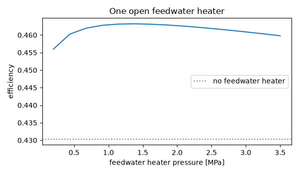
bleeds = np.linspace(0.2e6, 3.5e6, 15)
fig, ax = plt.subplots(figsize=(6, 3.5))
ax.plot(bleeds / 1e6, [rankine_cycle(15e6, 10e3, 873.15, feedwater_pressure=p).efficiency for p in bleeds])
ax.axhline(plants["simple"].efficiency, color="gray", ls=":", label="no feedwater heater")
ax.set(xlabel="feedwater heater pressure [MPa]", ylabel="efficiency", title="One open feedwater heater")
ax.legend()
fig.tight_layout()

plt.show()

real plant η = 0.428; Carnot between 600 °C and the condenser 0.635