Reeves’s pulse-code modulation (1937-1938)

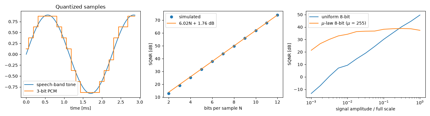
Alec Reeves, an engineer at International Telephone and Telegraph’s Paris laboratory, proposed sampling a speech waveform, rounding each sample to one of \(2^N\) levels and sending the level number as \(N\) on-off pulses (pcm_encode(), pcm_decode()). Rounding adds a small, fixed amount of noise, about \(6.02N + 1.76\) dB below a full-scale sine (pcm_sqnr_db()). In exchange, a repeater has only to decide whether each pulse is present, so noise does not accumulate along the line. The vacuum tubes of 1938 made PCM impractical. It waited for the transistor and the Bell System’s T1 carrier of 1962, which used companding (mu_law_compress()) to keep quiet speech above the quantization noise.

import matplotlib.pyplot as plt
import numpy as np

from engineeringkit.communications import mu_law_compress, mu_law_expand, pcm_decode, pcm_encode, pcm_sqnr_db

Sample, quantize, code

fs, f = 8000.0, 440.0
t = np.arange(24) / fs
x = 0.9 * np.sin(2 * np.pi * f * t)
bits = pcm_encode(x, 3)
y = pcm_decode(bits, 3)
print("first samples:", np.round(x[:4], 3).tolist())
print("3-bit words  :", ["".join(map(str, w)) for w in bits.reshape(-1, 3)[:4]])
assert np.max(np.abs(y - x)) <= 2 / 2**3 / 2

first samples: [0.0, 0.305, 0.574, 0.775]
3-bit words  : ['100', '101', '110', '111']

Six decibels per bit

n = np.arange(100_000)
sine = np.sin(2 * np.pi * 0.0123457 * n)
resolutions = np.arange(2, 13)
measured = [10 * np.log10(0.5 / np.mean((pcm_decode(pcm_encode(sine, N), N) - sine) ** 2)) for N in resolutions]
theory = [pcm_sqnr_db(N) for N in resolutions]
for N, m_db, t_db in zip(resolutions[::3], measured[::3], theory[::3]):
    print(f"N = {N:2d}: measured {m_db:5.2f} dB, 6.02N + 1.76 = {t_db:5.2f} dB")
assert np.allclose(measured[4:], theory[4:], atol=0.3)

N =  2: measured 12.81 dB, 6.02N + 1.76 = 13.80 dB
N =  5: measured 31.60 dB, 6.02N + 1.76 = 31.86 dB
N =  8: measured 49.66 dB, 6.02N + 1.76 = 49.93 dB
N = 11: measured 67.96 dB, 6.02N + 1.76 = 67.99 dB

Regeneration against analog accumulation

Send the same signal over 20 noisy hops. An analog repeater amplifies the noise along with the signal; a PCM repeater re-decides each pulse.

rng = np.random.default_rng(1938)
hops, sigma = 20, 0.06
analog = sine[:4000].copy()
pulses = pcm_encode(sine[:4000], 8)
for _ in range(hops):
    analog = analog + sigma * rng.standard_normal(analog.size)
    pulses = ((2.0 * pulses - 1 + 2 * sigma * rng.standard_normal(pulses.size)) > 0).astype(int)
snr_analog = 10 * np.log10(0.5 / np.mean((analog - sine[:4000]) ** 2))
snr_pcm = 10 * np.log10(0.5 / np.mean((pcm_decode(pulses, 8) - sine[:4000]) ** 2))
print(f"after {hops} hops: analog {snr_analog:.1f} dB, 8-bit PCM {snr_pcm:.1f} dB")
assert snr_pcm > snr_analog + 15

after 20 hops: analog 8.5 dB, 8-bit PCM 49.8 dB

Mu-law companding keeps quiet signals usable

levels = np.logspace(-3, 0, 13)
uniform, companded = [], []
for a in levels:
    s = a * sine
    uniform.append(10 * np.log10(np.mean(s**2) / np.mean((pcm_decode(pcm_encode(s, 8), 8) - s) ** 2)))
    out = mu_law_expand(pcm_decode(pcm_encode(mu_law_compress(s), 8), 8))
    companded.append(10 * np.log10(np.mean(s**2) / np.mean((out - s) ** 2)))
assert companded[0] > uniform[0] + 20 and np.ptp(companded[2:]) < 12

fig, axes = plt.subplots(1, 3, figsize=(14, 3.8))
tt = np.linspace(0, t[-1], 500)
axes[0].plot(tt * 1e3, 0.9 * np.sin(2 * np.pi * f * tt), label="speech-band tone")
axes[0].step(t * 1e3, y, where="mid", label="3-bit PCM")
axes[0].set(xlabel="time [ms]", title="Quantized samples")
axes[0].legend()
axes[1].plot(resolutions, measured, "o", label="simulated")
axes[1].plot(resolutions, theory, label="6.02N + 1.76 dB")
axes[1].set(xlabel="bits per sample N", ylabel="SQNR [dB]")
axes[1].legend()
axes[2].semilogx(levels, uniform, label="uniform 8-bit")
axes[2].semilogx(levels, companded, label=r"$\mu$-law 8-bit ($\mu$ = 255)")
axes[2].set(xlabel="signal amplitude / full scale", ylabel="SQNR [dB]")
axes[2].legend()
fig.tight_layout()

plt.show()