Delta modulation (1946-1952)

PCM needs an accurate multilevel coder. Delta modulation needs one comparator. The encoder keeps a staircase copy of the signal and sends a single bit per sample: 1 to step up by \(\Delta\), 0 to step down (delta_modulate()). The decoder rebuilds the staircase (delta_demodulate()) and smooths it. The idea appears in a 1946 French patent by Maurice Deloraine and colleagues at ITT’s Paris laboratory; Frank de Jager of Philips gave the first full published analysis in 1952. The step size is a compromise: small steps fall behind fast signals (slope overload, beyond \(\Delta f_s\), delta_slope_limit()), large steps leave granular noise where the signal is flat.

import matplotlib.pyplot as plt
import numpy as np

from engineeringkit.communications import delta_demodulate, delta_modulate, delta_slope_limit

Tracking, overload and granular noise

fs, f, A = 32e3, 400.0, 1.0
t = np.arange(400) / fs
x = A * np.sin(2 * np.pi * f * t)
needed = 2 * np.pi * f * A
fig, axes = plt.subplots(1, 3, figsize=(14, 3.8))
for ax, step, name in zip(axes[:2], (0.03, 0.1), ("slope overload", "tracking")):
    staircase = delta_demodulate(delta_modulate(x, step), step)
    ax.plot(t * 1e3, x, label="signal")
    ax.step(t * 1e3, staircase, where="post", label="staircase")
    limit = float(delta_slope_limit(step, fs))
    ax.set(xlabel="time [ms]", title=f"{name}: step {step}, limit {limit:.0f}/s vs {needed:.0f}/s")
    ax.legend()
    error = np.max(np.abs(staircase[:-1] - x[1:]))
    print(f"step {step}: slope limit {limit:.0f} per s, worst error {error:.3f}")
    assert (limit < needed) == (error > 3 * step)

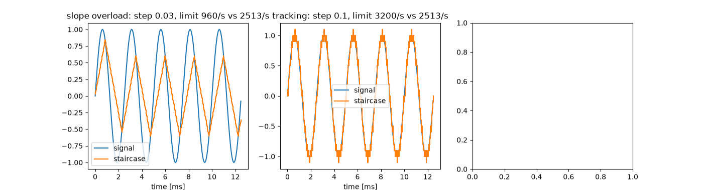
step 0.03: slope limit 960 per s, worst error 0.954
step 0.1: slope limit 3200 per s, worst error 0.178

The best step balances the two errors

steps = np.logspace(-2.5, -0.5, 41)
noise = []
for step in steps:
    staircase = delta_demodulate(delta_modulate(x, step), step)
    noise.append(np.mean((staircase[:-1] - x[1:]) ** 2))
noise = np.array(noise)
best = steps[np.argmin(noise)]
axes[2].loglog(steps, noise)
axes[2].axvline(needed / fs, color="k", ls=":", label=r"$\Delta = 2\pi f A / f_s$")
axes[2].axvline(best, color="C3", label="minimum")
axes[2].set(xlabel=r"step $\Delta$", ylabel="mean-square error", title="Overload (left) vs granular noise (right)")
axes[2].legend()
fig.tight_layout()
print(f"overload boundary {needed / fs:.3f}, best step {best:.3f}")
assert needed / fs < best < 3 * needed / fs

plt.show()

overload boundary 0.079, best step 0.079