Rayleigh’s sum of random phasors (1880)

Lord Rayleigh asked what amplitude results when a large number of vibrations of the same pitch but arbitrary phase are added, a question from optics and acoustics. The answer is a density \(f(r) = (2r/\Omega)e^{-r^2/\Omega}\), now called the Rayleigh distribution (rayleigh_pdf()). Seventy years later it described the mobile radio channel: a signal reaching a car by many scattered paths fades deeply and often. Averaged over the fades, the bit-error rate of BPSK falls only as \(1/4\bar\gamma\) (ber_bpsk_rayleigh()) instead of exponentially, so a fading link needs tens of decibels more power than a steady one.

import matplotlib.pyplot as plt
import numpy as np

from engineeringkit.communications import ber_bpsk_awgn, ber_bpsk_rayleigh, bpsk, from_db, rayleigh_pdf

Many random phasors make a Rayleigh envelope

rng = np.random.default_rng(1880)
paths, trials = 50, 100_000
phases = rng.uniform(0, 2 * np.pi, (trials, paths))
envelope = np.abs(np.sum(np.exp(1j * phases), axis=1)) / np.sqrt(paths)
r = np.linspace(0, 3.5, 200)
counts, edges = np.histogram(envelope, bins=60, range=(0, 3.5), density=True)
centres = (edges[1:] + edges[:-1]) / 2
print(f"mean square envelope {np.mean(envelope**2):.3f} (Rayleigh with Omega = 1)")
assert np.allclose(counts, rayleigh_pdf(centres), atol=0.03)
fades = np.mean(envelope**2 < 0.1)
print(f"time spent more than 10 dB below the mean: {fades:.3f} (theory 1 - exp(-0.1) = {1 - np.exp(-0.1):.3f})")
assert abs(fades - (1 - np.exp(-0.1))) < 0.005

mean square envelope 1.003 (Rayleigh with Omega = 1)
time spent more than 10 dB below the mean: 0.095 (theory 1 - exp(-0.1) = 0.095)

Fading costs tens of decibels

ebn0_db = np.arange(0, 31, 3.0)
n = 200_000
bits = rng.integers(0, 2, n)
measured = []
for g in from_db(ebn0_db):
    h = (rng.standard_normal(n) + 1j * rng.standard_normal(n)) / np.sqrt(2)
    y = h * bpsk(bits) + (rng.standard_normal(n) + 1j * rng.standard_normal(n)) * np.sqrt(1 / (2 * g))
    measured.append(np.mean((np.real(np.conj(h) * y) > 0) != bits))
theory = ber_bpsk_rayleigh(from_db(ebn0_db))
assert np.allclose(np.array(measured)[theory > 5e-3], theory[theory > 5e-3], rtol=0.1)
grid = np.linspace(0, 60, 6001)
need_fading = grid[np.argmax(ber_bpsk_rayleigh(from_db(grid)) < 1e-4)]
need_awgn = grid[np.argmax(ber_bpsk_awgn(from_db(grid)) < 1e-4)]
print(f"Eb/N0 for BER 1e-4: steady channel {need_awgn:.1f} dB, Rayleigh fading {need_fading:.1f} dB")
assert need_fading - need_awgn > 25

fig, axes = plt.subplots(1, 2, figsize=(11, 3.8))
axes[0].bar(centres, counts, width=edges[1] - edges[0], alpha=0.5, label=f"{paths} random phasors")
axes[0].plot(r, rayleigh_pdf(r), "C3", label=r"Rayleigh, $\Omega = 1$")
axes[0].set(xlabel="envelope r", ylabel="density")
axes[0].legend()
fine = np.linspace(0, 30, 301)
axes[1].semilogy(fine, ber_bpsk_awgn(from_db(fine)), label="steady (AWGN)")
axes[1].semilogy(fine, ber_bpsk_rayleigh(from_db(fine)), label="Rayleigh fading")
axes[1].semilogy(ebn0_db, measured, "k.", label="simulation")
axes[1].set(xlabel=r"mean $E_b/N_0$ [dB]", ylabel="bit-error rate", ylim=(1e-6, 0.5))
axes[1].grid(True, which="both", alpha=0.3)
axes[1].legend()
fig.tight_layout()

plt.show()

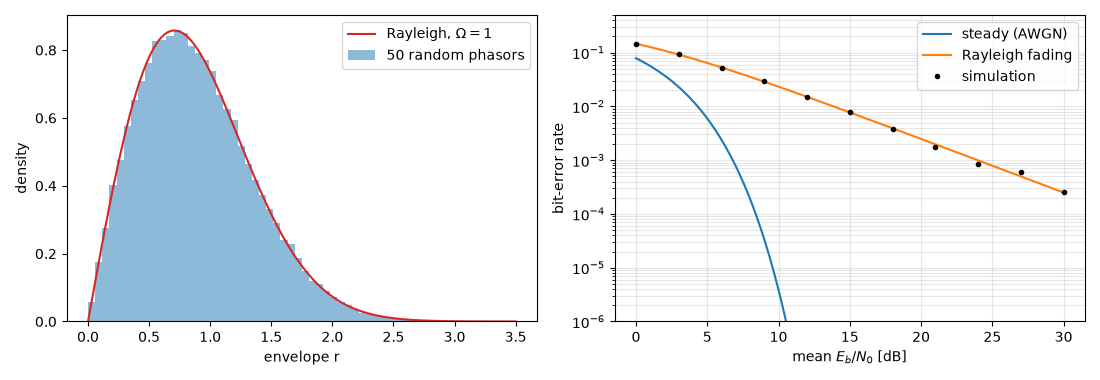
Eb/N0 for BER 1e-4: steady channel 8.4 dB, Rayleigh fading 34.0 dB