Kahn and Brennan’s diversity combining (1954-1959)

Two antennas a few wavelengths apart rarely fade at the same moment. Short-wave receivers had long switched to whichever antenna was strongest (selection, selection_outage_probability()). Leonard Kahn’s 1954 “ratio squarer” instead weighted each branch by its own signal strength before adding them. With complex weights equal to the conjugate channel gains this is maximal-ratio combining (maximal_ratio_combine()), whose output SNR is the sum of the branch SNRs. D. G. Brennan’s 1959 review compared selection, equal-gain and maximal-ratio combining and showed how close they come to one another. With \(L\) independent branches the error rate falls as \(\bar\gamma^{-L}\) (ber_bpsk_mrc_rayleigh()).

import matplotlib.pyplot as plt
import numpy as np

from engineeringkit.communications import ber_bpsk_mrc_rayleigh, bpsk, from_db, maximal_ratio_combine, selection_outage_probability

Maximal-ratio combining by simulation

rng = np.random.default_rng(1954)
ebn0_db = np.arange(0, 25, 3.0)
n = 200_000
bits = rng.integers(0, 2, n)
fig, axes = plt.subplots(1, 2, figsize=(11, 3.8))
fine = np.linspace(0, 25, 251)
for L in (1, 2, 4):
    measured = []
    for g in from_db(ebn0_db):
        h = (rng.standard_normal((L, n)) + 1j * rng.standard_normal((L, n))) / np.sqrt(2)
        y = h * bpsk(bits) + (rng.standard_normal((L, n)) + 1j * rng.standard_normal((L, n))) * np.sqrt(1 / (2 * g))
        measured.append(np.mean((np.real(maximal_ratio_combine(y, h)) > 0) != bits))
    measured = np.array(measured)
    theory = ber_bpsk_mrc_rayleigh(from_db(ebn0_db), L)
    reliable = theory > 1e-4
    assert np.allclose(measured[reliable], theory[reliable], rtol=0.15)
    axes[0].semilogy(fine, ber_bpsk_mrc_rayleigh(from_db(fine), L), label=f"L = {L}")
    axes[0].semilogy(ebn0_db[measured > 0], measured[measured > 0], "k.")
    slope = np.log10(ber_bpsk_mrc_rayleigh(1e2, L) / ber_bpsk_mrc_rayleigh(1e3, L))
    print(f"L = {L}: BER at 10 dB = {ber_bpsk_mrc_rayleigh(10.0, L):.2e}, decades per decade of SNR = {slope:.2f}")
    assert abs(slope - L) < 0.1
axes[0].set(xlabel=r"mean $E_b/N_0$ per branch [dB]", ylabel="bit-error rate", ylim=(1e-6, 0.5), title="Maximal-ratio combining")
axes[0].grid(True, which="both", alpha=0.3)
axes[0].legend()

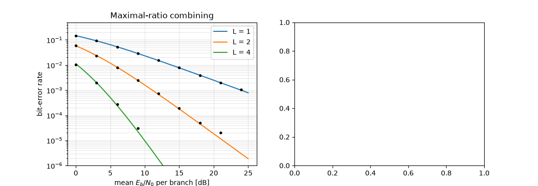
L = 1: BER at 10 dB = 2.33e-02, decades per decade of SNR = 1.00
L = 2: BER at 10 dB = 1.60e-03, decades per decade of SNR = 1.99
L = 4: BER at 10 dB = 9.70e-06, decades per decade of SNR = 3.99

<matplotlib.legend.Legend object at 0x7f97828c5c40>

Selection diversity and outage

threshold = from_db(np.linspace(-30, 10, 201))
for L in (1, 2, 4):
    axes[1].semilogy(10 * np.log10(threshold), selection_outage_probability(threshold, 1.0, L), label=f"L = {L}")
gains = np.abs((rng.standard_normal((2, n)) + 1j * rng.standard_normal((2, n))) / np.sqrt(2)) ** 2
measured_outage = np.mean(np.max(gains, axis=0) < 0.1)
print(f"two-branch selection, 10 dB below the mean: outage {measured_outage:.4f}, theory {selection_outage_probability(0.1, 1.0, 2):.4f}")
assert abs(measured_outage - selection_outage_probability(0.1, 1.0, 2)) < 0.002
axes[1].set(xlabel="threshold relative to mean SNR [dB]", ylabel="outage probability", title="Selection combining", ylim=(1e-6, 1))
axes[1].grid(True, which="both", alpha=0.3)
axes[1].legend()
fig.tight_layout()

plt.show()

two-branch selection, 10 dB below the mean: outage 0.0090, theory 0.0091