Watt’s centrifugal governor and proportional droop

James Watt’s flyball governor (1788) closed the steam valve as the engine sped up: the throttle moved in proportion to the speed error. Model the engine as \(J\dot\omega = \tau - b\omega - \tau_{load}\) and the governor as \(\tau = K_p(\omega_{ref} - \omega)\), a proportional PID. A proportional governor holds speed far better than an open throttle, but it always leaves a steady droop, \(\Delta\omega = \tau_{load}/(b + K_p)\), which shrinks with gain but never vanishes.

import matplotlib.pyplot as plt
import numpy as np

from engineeringkit.control_systems import PID, dc_gain, feedback, step_response, transfer_function

J, b = 2.0, 0.5  # inertia [kg m^2], friction [N m s]
engine = transfer_function([1], [J, b])  # speed per unit torque

Response to a sudden load

The load torque enters at the plant input, so the speed disturbance is \(G/(1 + GC)\).

t = np.linspace(0, 40, 1601)
load = 1.0
fig, ax = plt.subplots()
for kp in [0.0, 2.0, 8.0, 32.0]:
    to_speed = feedback(engine, PID(kp).transfer_function()) if kp else engine
    _, dw = step_response(to_speed, t)
    droop = -load * dc_gain(to_speed)
    assert np.isclose(droop, -load / (b + kp))
    assert np.isclose(-load * dw[-1], droop, rtol=1e-3)
    ax.plot(t, -load * dw, label=f"$K_p$ = {kp:g}: droop {droop:.3f} rad/s")
    print(f"K_p = {kp:5.1f}: steady speed change {droop:.4f} rad/s")
ax.set(xlabel="time [s]", ylabel="speed change [rad/s]", title="Engine speed after a 1 N m load step")
ax.legend()

plt.show()

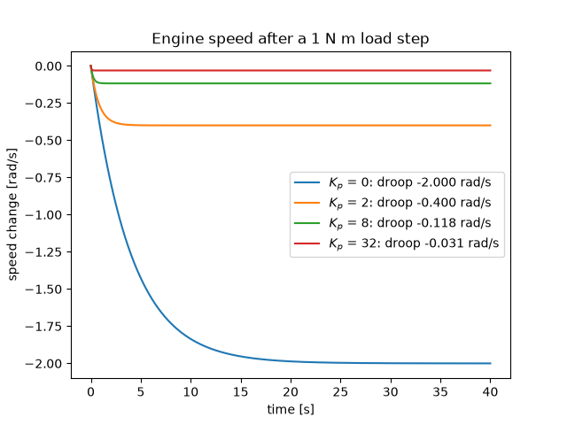
K_p =   0.0: steady speed change -2.0000 rad/s
K_p =   2.0: steady speed change -0.4000 rad/s
K_p =   8.0: steady speed change -0.1176 rad/s
K_p =  32.0: steady speed change -0.0308 rad/s