Black’s negative-feedback amplifier

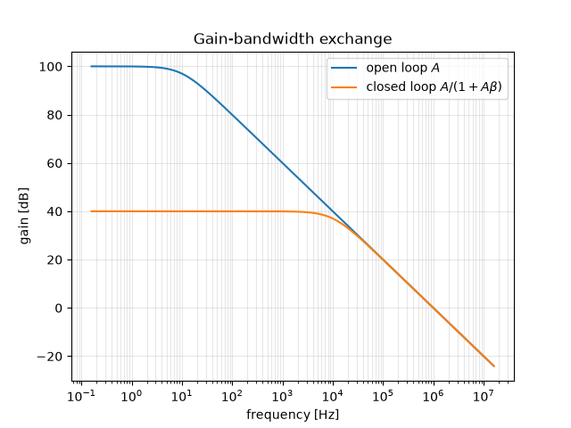
Harold Black (1927), commuting on the Lackawanna ferry, sketched an amplifier that fed a fraction \(\beta\) of its output back out of phase. With a huge open-loop gain \(A\), the closed-loop gain \(A/(1 + A\beta)\) (feedback()) is almost exactly \(1/\beta\), set by a passive divider rather than by drifting vacuum tubes. Distortion and gain variations shrink by the factor \(1 + A\beta\), and the bandwidth grows by the same factor.

import matplotlib.pyplot as plt
import numpy as np

from engineeringkit.control_systems import bode, dc_gain, feedback, poles, transfer_function

beta = 0.01
wa = 2 * np.pi * 10.0  # open-loop pole [rad/s]

Insensitivity to the tube gain

for A0 in [5e4, 1e5, 1.5e5]:
    amp = transfer_function([A0], [1 / wa, 1])
    closed = feedback(amp, beta)
    gain = dc_gain(closed)
    print(f"A0 = {A0:8.0f}: closed-loop gain {gain:.4f}, bandwidth {-poles(closed)[0].real / (2 * np.pi):8.0f} Hz")
    assert np.isclose(-poles(closed)[0].real, wa * (1 + A0 * beta))
    assert np.isclose(gain, A0 / (1 + A0 * beta)) and abs(gain * beta - 1) < 2.5e-3

A0 =    50000: closed-loop gain 99.8004, bandwidth     5010 Hz
A0 =   100000: closed-loop gain 99.9001, bandwidth    10010 Hz
A0 =   150000: closed-loop gain 99.9334, bandwidth    15010 Hz

Gain traded for bandwidth

amp = transfer_function([1e5], [1 / wa, 1])
w = np.logspace(0, 8, 400)
fig, ax = plt.subplots()
for model, label in [(amp, "open loop $A$"), (feedback(amp, beta), r"closed loop $A/(1+A\beta)$")]:
    _, mag, _ = bode(model, w)
    ax.semilogx(w / (2 * np.pi), mag, label=label)
ax.set(xlabel="frequency [Hz]", ylabel="gain [dB]", title="Gain-bandwidth exchange")
ax.grid(True, which="both", alpha=0.3)
ax.legend()

plt.show()