Nyquist’s stability criterion

Long-distance telephone repeaters with feedback sometimes “sang”. Harry Nyquist (1932) showed how to predict this from the measured open-loop frequency response alone. Trace \(L(j\omega)\) for all frequencies (nyquist()): the closed loop has \(Z = N + P\) unstable poles, where \(N\) counts clockwise encirclements of \(-1\) (nyquist_encirclements()) and \(P\) the unstable open-loop poles.

import matplotlib.pyplot as plt
import numpy as np

from engineeringkit.control_systems import feedback, nyquist_encirclements, poles, transfer_function
from engineeringkit.control_systems.visualizers import plot_nyquist

A stable plant at two gains

\(K/(s+1)^3\) crosses the negative real axis at \(-K/8\).

fig, axes = plt.subplots(1, 2, figsize=(10, 4))
for K in [4.0, 12.0]:
    loop = transfer_function([K], [1, 3, 3, 1])
    N = nyquist_encirclements(loop)
    Z = int(np.sum(poles(feedback(loop)).real > 0))
    print(f"K = {K:4.1f}: N = {N}, P = 0, closed-loop unstable poles Z = {Z}")
    assert Z == N + 0
    plot_nyquist(loop, ax=axes[0], label=f"K = {K:g}, N = {N}")
axes[0].set(xlim=(-3, 13), ylim=(-8, 8), title=r"$K/(s+1)^3$")

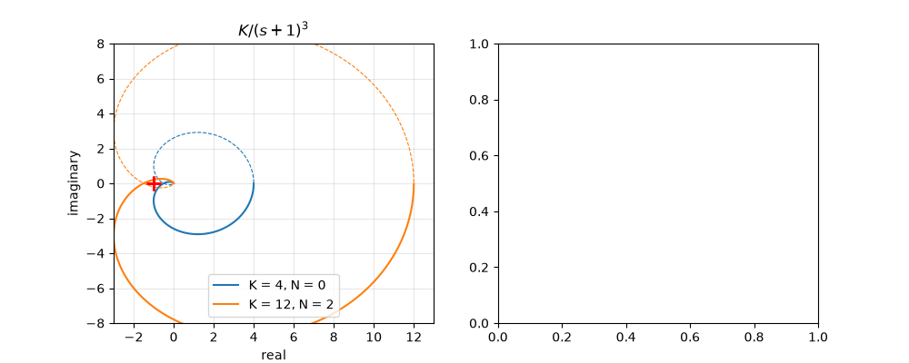
K =  4.0: N = 0, P = 0, closed-loop unstable poles Z = 0
K = 12.0: N = 2, P = 0, closed-loop unstable poles Z = 2

[(-3.0, 13.0), (-8.0, 8.0), Text(0.5, 1.0, '$K/(s+1)^3$')]

An unstable plant stabilised by feedback

\(2/(s-1)\) has one unstable pole (\(P = 1\)); one counter-clockwise encirclement (\(N = -1\)) gives \(Z = 0\).

loop = transfer_function([2], [1, -1])
N = nyquist_encirclements(loop)
Z = int(np.sum(poles(feedback(loop)).real > 0))
print(f"2/(s-1): N = {N}, P = 1, Z = {Z}")
assert N == -1 and Z == N + 1
plot_nyquist(loop, ax=axes[1], label="$2/(s-1)$")
axes[1].set(title="Unstable open loop, stable closed loop")
axes[1].set_aspect("equal")
fig.tight_layout()

plt.show()

2/(s-1): N = -1, P = 1, Z = 0