Kalman’s controllability and observability (1960)

A transfer function describes only the part of a system that the input reaches and the output sees. Rudolf Kalman (1960) split the state into these parts. The state of \(\dot x = Ax + Bu\) can be steered anywhere only if the controllability matrix \([B, AB, \dots, A^{n-1}B]\) has full rank, and reconstructed from \(y = Cx\) only if the observability matrix \([C; CA; \dots; CA^{n-1}]\) does (is_controllable(), is_observable()). A mode that fails either test disappears from the transfer function in a pole-zero cancellation, but it is still there.

import matplotlib.pyplot as plt
import numpy as np
from scipy import signal
from scipy.integrate import solve_ivp

from engineeringkit.control_systems import (
    controllability_matrix,
    is_controllable,
    is_observable,
    observability_matrix,
)

An uncontrollable pair of tanks

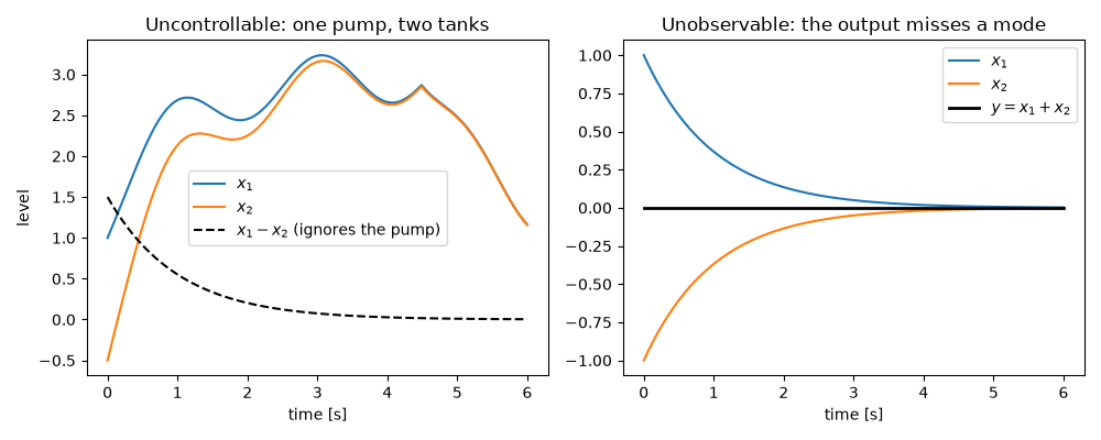
Two identical tanks, \(\dot x_i = -x_i + u\), are filled by the same pump. Whatever the pump does, the difference \(x_1 - x_2\) decays as \(e^{-t}\) on its own.

A1, B1 = -np.eye(2), np.array([[1.0], [1.0]])
print("rank of [B, AB] =", np.linalg.matrix_rank(controllability_matrix(A1, B1)))
assert not is_controllable(A1, B1)


def pump(t):
    return 2 + np.sin(3 * t) + np.sign(np.sin(0.7 * t))


tt = np.linspace(0, 6, 601)
x0 = [1.0, -0.5]
tanks = solve_ivp(lambda t, x: A1 @ x + B1[:, 0] * pump(t), (0, 6), x0, t_eval=tt, rtol=1e-10, atol=1e-12)
difference = tanks.y[0] - tanks.y[1]
assert np.allclose(difference, (x0[0] - x0[1]) * np.exp(-tt), atol=1e-8)

rank of [B, AB] = 1

An unobservable mode hidden by a cancellation

For \(A = [[0, 1], [-2, -3]]\) (modes \(-1\) and \(-2\)), \(B = [0, 1]^\mathsf{T}\) and \(C = [1, 1]\), the output never sees the \(-1\) mode: the transfer function is \((s+1)/((s+1)(s+2)) = 1/(s+2)\). Starting on that mode’s eigenvector the state moves while the output stays exactly zero.

A2, B2, C2 = np.array([[0.0, 1.0], [-2.0, -3.0]]), np.array([[0.0], [1.0]]), np.array([[1.0, 1.0]])
assert is_controllable(A2, B2) and not is_observable(A2, C2)
print("rank of [C; CA] =", np.linalg.matrix_rank(observability_matrix(A2, C2)))
num, den = signal.ss2tf(A2, B2, C2, [[0.0]])
print("transfer function zeros:", np.roots(num[0]).round(6), "poles:", np.roots(den).round(6))
assert np.isclose(np.roots(num[0])[0], -1) and np.min(np.abs(np.roots(den) + 1)) < 1e-9

hidden = solve_ivp(lambda t, x: A2 @ x, (0, 6), [1.0, -1.0], t_eval=tt, rtol=1e-10, atol=1e-12)
y_hidden = C2 @ hidden.y
assert np.abs(y_hidden).max() < 1e-8 and np.abs(hidden.y).max() > 0.9
C3 = np.array([[1.0, 0.0]])  # measure x1 alone and both modes are visible
assert is_observable(A2, C3)

fig, (ax1, ax2) = plt.subplots(1, 2, figsize=(10, 4))
ax1.plot(tt, tanks.y[0], label="$x_1$")
ax1.plot(tt, tanks.y[1], label="$x_2$")
ax1.plot(tt, difference, "k--", label="$x_1 - x_2$ (ignores the pump)")
ax1.set(xlabel="time [s]", ylabel="level", title="Uncontrollable: one pump, two tanks")
ax1.legend()
ax2.plot(tt, hidden.y[0], label="$x_1$")
ax2.plot(tt, hidden.y[1], label="$x_2$")
ax2.plot(tt, y_hidden[0], "k-", lw=2, label="$y = x_1 + x_2$")
ax2.set(xlabel="time [s]", title="Unobservable: the output misses a mode")
ax2.legend()
fig.tight_layout()

plt.show()

rank of [C; CA] = 1
transfer function zeros: [-1.] poles: [-2. -1.]