Hazen’s theory of servomechanisms

Harold Hazen at MIT (1934) coined servomechanism and analysed position-following systems as second-order dynamics, \(\omega_n^2/(s^2 + 2\zeta\omega_n s + \omega_n^2)\). The damping ratio \(\zeta\) alone fixes the overshoot, and \(\zeta\) with the natural frequency \(\omega_n\) sets peak and settling times (second_order_metrics()). The simulated step and impulse responses (step_response(), impulse_response()) confirm the formulas.

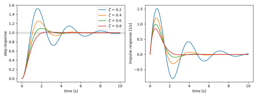
zeta=0.2: overshoot 52.66% (formula 52.66%), settling 9.80 s (estimate 10.00 s)
zeta=0.4: overshoot 25.38% (formula 25.38%), settling 4.20 s (estimate 5.00 s)
zeta=0.6: overshoot  9.48% (formula  9.48%), settling 2.97 s (estimate 3.33 s)
zeta=0.8: overshoot  1.52% (formula  1.52%), settling 1.88 s (estimate 2.50 s)

import matplotlib.pyplot as plt
import numpy as np

from engineeringkit.control_systems import impulse_response, second_order_metrics, step_response, transfer_function

wn = 2.0
t = np.linspace(0, 10, 20001)
fig, axes = plt.subplots(1, 2, figsize=(10, 3.8))
for zeta in [0.2, 0.4, 0.6, 0.8]:
    servo = transfer_function([wn**2], [1, 2 * zeta * wn, wn**2])
    _, y = step_response(servo, t)
    _, h = impulse_response(servo, t)
    spec = second_order_metrics(zeta, wn)
    overshoot, peak_time = 100 * (y.max() - 1), t[np.argmax(y)]
    settled = t[np.flatnonzero(np.abs(y - 1) > 0.02)[-1]]
    print(
        f"zeta={zeta}: overshoot {overshoot:5.2f}% (formula {spec['percent_overshoot']:5.2f}%), "
        f"settling {settled:.2f} s (estimate {spec['settling_time_2pct']:.2f} s)"
    )
    assert abs(overshoot - spec["percent_overshoot"]) < 0.01 and abs(peak_time - spec["peak_time"]) < 1e-3
    # The impulse response is the derivative of the step response; it first crosses zero at the peak.
    assert abs(t[np.argmax(h < 0)] - spec["peak_time"]) < 1e-3
    axes[0].plot(t, y, label=rf"$\zeta$ = {zeta}")
    axes[1].plot(t, h, label=rf"$\zeta$ = {zeta}")
axes[0].axhspan(0.98, 1.02, color="gray", alpha=0.2)
axes[0].set(xlabel="time [s]", ylabel="step response")
axes[1].set(xlabel="time [s]", ylabel="impulse response [1/s]")
axes[0].legend()
fig.tight_layout()

plt.show()