Smith’s predictor for dead time (1957)

A chemical plant often measures its output only after a transport delay \(\theta\): the time for a fluid to reach the sensor. The delay adds phase lag \(\omega\theta\) at every frequency, so a controller tuned for the delay-free plant oscillates or goes unstable once the delay is added. Otto Smith (1957) put a model of the plant inside the controller. It feeds back the undelayed model output and corrects it by the mismatch between the measurement and the delayed model output. 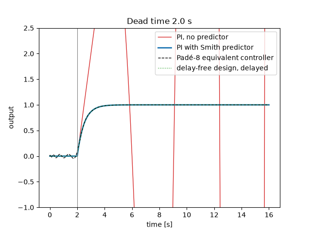With a perfect model the loop behaves like the delay-free design, delayed by \(\theta\) (smith_predictor()).

The plant here is \(G = 1/(s+1)\) with \(\theta = 2\) s, and the PI controller \(C = 2(1 + 1/s)\) cancels the plant pole, so the delay-free loop is \(T_0 = 2/(s+2)\).

import matplotlib.pyplot as plt
import numpy as np

from engineeringkit.control_systems import (
    feedback,
    pade_delay,
    poles,
    smith_predictor,
    stability_margins,
    step_response,
    transfer_function,
)

G = transfer_function([1], [1, 1])
C = transfer_function([2, 2], [1, 0])
theta, kp = 2.0, 2.0

The delay destroys the phase margin

The loop \(CG = 2/s\) crosses unity gain at 2 rad/s with a 90° margin. The delay subtracts \(2 \times 2\) rad, about 229°, so the plain PI loop is unstable. A high-order Padé approximant (pade_delay()) stands in for the delay in the margin calculation.

D = pade_delay(theta, order=8)
w = np.logspace(-2, 0.5, 400)
pade_phase = np.unwrap(np.angle(np.polyval(D.num, 1j * w) / np.polyval(D.den, 1j * w)))
assert np.allclose(np.abs(np.polyval(D.num, 1j * w) / np.polyval(D.den, 1j * w)), 1)  # all-pass
assert np.allclose(pade_phase, -w * theta, atol=1e-6)  # exact phase well below w*theta = 8
delayed_loop = transfer_function(np.polymul([2], D.num), np.polymul([1, 0], D.den))
pm = stability_margins(delayed_loop)["phase_margin_deg"]
print(f"phase margin: delay-free 90.0 deg, with the delay {pm:.1f} deg")
assert np.isclose(pm, 90 - np.degrees(kp * theta), atol=0.1)

phase margin: delay-free 90.0 deg, with the delay -139.2 deg

Simulating the true delay

A computer implements the delay as a buffer of past commands. The loop below runs plant, controller and model at a 1 ms step, once with the plain PI controller and once with the predictor.

dt = 1e-3
t = np.arange(0, 16, dt)
lag = round(theta / dt)


def simulate(predictor):
    y = np.zeros(t.size)
    x = xm = integral = 0.0  # plant, model and PI integrator states
    u_hist, ym_hist = np.zeros(t.size), np.zeros(t.size)
    for k in range(t.size - 1):
        ym_delayed = ym_hist[k - lag] if k >= lag else 0.0
        e = 1.0 - y[k] - (xm - ym_delayed if predictor else 0.0)
        u = kp * e + kp * integral
        integral += e * dt
        u_hist[k], ym_hist[k] = u, xm
        u_delayed = u_hist[k - lag] if k >= lag else 0.0
        x += (u_delayed - x) * dt
        xm += (u - xm) * dt
        y[k + 1] = x
    return y


y_plain, y_smith = simulate(False), simulate(True)
ideal = np.where(t > theta, 1 - np.exp(-kp * (t - theta)), 0.0)
print(f"Smith predictor vs delayed T0: max error {np.abs(y_smith - ideal).max():.4f}")
assert np.abs(y_smith - ideal).max() < 0.01
assert np.abs(y_plain[t > 8]).max() > 2  # the plain PI loop diverges

Smith predictor vs delayed T0: max error 0.0004

The equivalent controller

Folded into one transfer function, the predictor is \(C/(1 + CG(1 - e^{-s\theta}))\). Closing it around the Padé model of the delayed plant cancels the delay from the characteristic equation: the closed-loop poles are the delay-free pole \(-2\) plus poles that cancel against zeros.

Csp = smith_predictor(C, G, theta, order=8)
plant = transfer_function(D.num, np.polymul([1, 1], D.den))
loop = transfer_function(np.polymul(Csp.num, plant.num), np.polymul(Csp.den, plant.den))
closed = feedback(loop)
assert np.all(poles(closed).real < 0)
assert np.min(np.abs(poles(closed) + 2)) < 1e-6
_, y_pade = step_response(closed, t)
print(f"Padé-model predictor vs delayed T0: max error after the delay {np.abs(y_pade - ideal)[t > theta + 1].max():.4f}")
assert np.abs(y_pade - ideal)[t > theta + 1].max() < 0.01

fig, ax = plt.subplots()
ax.plot(t, y_plain, color="C3", lw=1, label="PI, no predictor")
ax.plot(t, y_smith, color="C0", lw=2, label="PI with Smith predictor")
ax.plot(t, y_pade, "k--", lw=1, label="Padé-8 equivalent controller")
ax.plot(t, ideal, color="C2", lw=1, ls=":", label="delay-free design, delayed")
ax.axvline(theta, color="gray", lw=0.8)
ax.set(xlabel="time [s]", ylabel="output", ylim=(-1, 2.5), title=f"Dead time {theta} s")
ax.legend(loc="upper right")

plt.show()

Padé-model predictor vs delayed T0: max error after the delay 0.0013