Ragazzini’s operational amplifier (1947)

Analog computers of the 1940s solved differential equations with high-gain DC amplifiers wrapped in resistive and capacitive feedback. John Ragazzini, Robert Randall and Frederick Russell of Columbia University analysed them in 1947 and named them operational amplifiers, because each performed a mathematical operation: with a large enough gain the feedback forces the inverting input to a virtual ground, so the output depends only on the feedback network. A resistor ratio scales and inverts (inverting_amplifier_gain()), the non-inverting connection scales without inversion (noninverting_amplifier_gain()) and a feedback capacitor integrates (op_amp_integrator()). This example checks the ideal gains against an amplifier of finite open-loop gain, then wires two integrators into a loop that solves \(\ddot y = -\omega^2 y\), as an analog computer did.

import matplotlib.pyplot as plt
import numpy as np

from engineeringkit.electrical_engineering import inverting_amplifier_gain, noninverting_amplifier_gain, op_amp_integrator

The ideal gains and a finite open-loop gain

With open-loop gain \(A\), the inverting amplifier gives \(-(R_f/R_i)/(1 + (1 + R_f/R_i)/A)\); the ideal value is the limit \(A \to \infty\).

Rf, Ri = 100e3, 10e3
ideal_inv, ideal_non = inverting_amplifier_gain(Rf, Ri), noninverting_amplifier_gain(Rf, Ri)
print(f"ideal gains: inverting {ideal_inv:.1f}, non-inverting {ideal_non:.1f}")
for A in (1e2, 1e4, 1e6):
    actual = -(Rf / Ri) / (1 + (1 + Rf / Ri) / A)
    print(f"A = {A:.0e}: inverting gain {actual:.4f} ({abs(actual / ideal_inv - 1):.2%} short)")
assert abs(-(Rf / Ri) / (1 + (1 + Rf / Ri) / 1e6) / ideal_inv - 1) < 2e-5

ideal gains: inverting -10.0, non-inverting 11.0
A = 1e+02: inverting gain -9.0090 (9.91% short)
A = 1e+04: inverting gain -9.9890 (0.11% short)
A = 1e+06: inverting gain -9.9999 (0.00% short)

Two integrators in a loop: an analog computer

Integrating \(\ddot y\) twice gives \(y\); feeding \(-\omega^2 y\) back as \(\ddot y\) closes the loop. Each inverting integrator flips the sign, so a unity-gain inverter (\(R_f = R_i\)) restores the minus sign of \(-\omega^2 y\); without it the loop would grow exponentially. The circuit is stepped forward in short intervals, each integrator integrating its sampled input.

R, C = 100e3, 1e-6  # RC = 0.1 s, so omega = 1/RC = 10 rad/s
omega = 1 / (R * C)
dt, n = 1e-4, 12000
t = np.arange(n) * dt
inverter = inverting_amplifier_gain(R, R)
y, u = np.empty(n), np.empty(n)
y[0], u[0] = 1.0, 0.0
for k in range(n - 1):
    span = t[k : k + 2]
    # First integrator: input y, output u = -(1/RC) int y dt.
    u[k + 1] = op_amp_integrator([y[k], y[k]], span, R, C, v0=u[k])[-1]
    # Inverter, then the second integrator: input -u, output y = (1/RC) int u dt.
    y[k + 1] = op_amp_integrator(inverter * u[[k + 1, k + 1]], span, R, C, v0=y[k])[-1]
print(f"after {t[-1]:.1f} s: y = {y[-1]:.4f}, exact cos(omega t) = {np.cos(omega * t[-1]):.4f}")
assert np.max(np.abs(y - np.cos(omega * t))) < 2e-2

fig, axes = plt.subplots(1, 2, figsize=(10, 3.6))
for A in (1e1, 1e2, 1e3):
    ratio = np.logspace(0, 3, 50)
    axes[0].semilogx(ratio, (ratio / (1 + (1 + ratio) / A)) / ratio, label=f"A = {A:.0e}")
axes[0].set(xlabel="ideal gain magnitude $R_f/R_i$", ylabel="actual / ideal", title="Finite open-loop gain")
axes[0].legend(fontsize="small")
axes[1].plot(t, y, label="integrator loop")
axes[1].plot(t, np.cos(omega * t), "k:", label="cos(omega t)")
axes[1].set(xlabel="time [s]", ylabel="output [V]", title="Two-integrator oscillator")
axes[1].legend(fontsize="small")
fig.tight_layout()

plt.show()

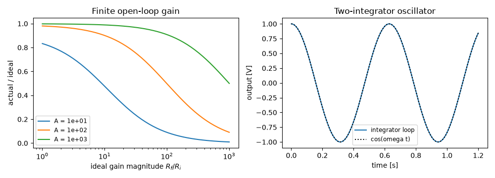
after 1.2 s: y = 0.8436, exact cos(omega t) = 0.8433