Shockley’s diode equation and the load line (1949)

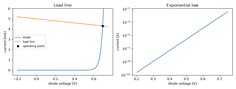
William Shockley’s theory of the p-n junction, published in 1949 with the junction transistor, explained why a diode conducts one way: minority carriers injected across the junction diffuse away at a rate that grows as \(e^{qv/kT}\), so the current is \(i = I_S\left(e^{v/nV_T} - 1\right)\) with the thermal voltage \(V_T = kT/q\) (shockley_diode_current(), thermal_voltage()). In a circuit the diode shares its current with a resistor, whose straight load line meets the exponential at the operating point (diode_operating_point()). This example draws the characteristic, solves a load line and checks the famous 60 mV per decade and the fall of the forward voltage with temperature, roughly 2 mV/K.

import matplotlib.pyplot as plt
import numpy as np

from engineeringkit.electrical_engineering import diode_operating_point, shockley_diode_current, thermal_voltage

The characteristic

Is, n = 1e-14, 1.0
vt = thermal_voltage(300.0)
v = np.linspace(-0.2, 0.75, 400)
i = shockley_diode_current(v, Is, n)
per_decade = n * vt * np.log(10)
print(f"V_T = {1e3 * vt:.2f} mV at 300 K; forward voltage rises {1e3 * per_decade:.1f} mV per decade of current")
assert np.isclose(shockley_diode_current(0.65 + per_decade, Is) / shockley_diode_current(0.65, Is), 10, rtol=1e-6)

V_T = 25.85 mV at 300 K; forward voltage rises 59.5 mV per decade of current

The load-line solution

A 5 V supply drives the diode through 1 kΩ.

Vs, R = 5.0, 1e3
vd, idiode = diode_operating_point(Vs, R, Is, n)
print(f"operating point: v = {vd:.4f} V, i = {1e3 * idiode:.4f} mA")
assert np.isclose(idiode, (Vs - vd) / R) and np.isclose(idiode, shockley_diode_current(vd, Is, n), rtol=1e-9)
# The constant-drop model a student would use is within a few percent.
print(f"0.7 V model: i = {1e3 * (Vs - 0.7) / R:.3f} mA")

operating point: v = 0.6925 V, i = 4.3075 mA
0.7 V model: i = 4.300 mA

Temperature

At a fixed current the forward voltage falls with temperature, because \(I_S\) grows much faster than \(V_T\) (roughly \(I_S \propto T^3 e^{-E_g/kT}\) with \(E_g = 1.12\) eV for silicon).

def saturation_current(T, Is300=Is, Eg=1.12):
    return Is300 * (T / 300) ** 3 * np.exp(Eg / (n * thermal_voltage(300.0)) - Eg / (n * thermal_voltage(T)))


temperatures = np.array([280.0, 300.0, 320.0])
forward = [diode_operating_point(Vs, R, saturation_current(T), n, T)[0] for T in temperatures]
slope = np.polyfit(temperatures, forward, 1)[0]
print(f"forward voltage temperature coefficient {1e3 * slope:.2f} mV/K")
assert -2.5e-3 < slope < -1.5e-3

fig, axes = plt.subplots(1, 2, figsize=(10, 3.8))
axes[0].plot(v, 1e3 * i, label="diode")
axes[0].plot(v, 1e3 * (Vs - v) / R, label="load line")
axes[0].plot(vd, 1e3 * idiode, "ko", label="operating point")
axes[0].set(xlabel="diode voltage [V]", ylabel="current [mA]", ylim=(-0.5, 6), title="Load line")
axes[0].legend(fontsize="small")
axes[1].semilogy(v[v > 0.2], i[v > 0.2])
axes[1].set(xlabel="diode voltage [V]", ylabel="current [A]", title="Exponential law")
fig.tight_layout()

plt.show()

forward voltage temperature coefficient -1.67 mV/K