Kelvin’s oscillatory discharge and the RLC step response (1853)

Felix Savary and Joseph Henry had seen that a Leyden jar discharged through a coil could magnetise needles either way, as if the current reversed. In 1853 William Thomson (later Lord Kelvin) wrote down the equation of the discharge, a capacitance, an inductance and a resistance in series, and found that it is a single surge if \(R > 2\sqrt{L/C}\) and an oscillation of period close to \(2\pi\sqrt{LC}\) if it is less. Feddersen photographed the oscillating spark a few years later. In modern terms the series RLC circuit has the neper frequency \(\alpha = R/2L\) and the resonant frequency \(\omega_0 = 1/\sqrt{LC}\), and is over-, critically or underdamped as \(\alpha\) is larger than, equal to or smaller than \(\omega_0\) (rlc_damping(), rlc_step_voltage()). This example shows the three regimes of the step response and checks the ringing frequency and decay of the underdamped one.

import matplotlib.pyplot as plt
import numpy as np

from engineeringkit.electrical_engineering import rlc_damping, rlc_step_voltage

The three regimes

A 1 mH, 1 µF circuit is critically damped at \(R = 2\sqrt{L/C}\).

L, C = 1e-3, 1e-6
R_critical = 2 * np.sqrt(L / C)
t = np.linspace(0, 1.2e-3, 4001)
fig, ax = plt.subplots(figsize=(7, 3.8))
for R in (4 * R_critical, R_critical, 0.1 * R_critical):
    alpha, omega0, regime = rlc_damping(R, L, C)
    v = rlc_step_voltage(1.0, R, L, C, t)
    print(f"R = {R:6.1f} ohm: alpha = {alpha:8.0f} 1/s, omega0 = {omega0:6.0f} rad/s, {regime}, overshoot {max(v.max() - 1, 0):.1%}")
    ax.plot(1e3 * t, v, label=f"R = {R:.0f} ohm ({regime})")
assert rlc_damping(R_critical, L, C)[2] == "critically damped"

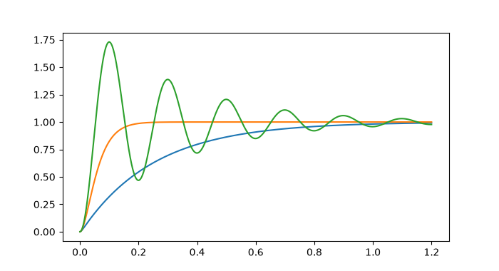
R =  253.0 ohm: alpha =   126491 1/s, omega0 =  31623 rad/s, overdamped, overshoot 0.0%
R =   63.2 ohm: alpha =    31623 1/s, omega0 =  31623 rad/s, critically damped, overshoot 0.0%
R =    6.3 ohm: alpha =     3162 1/s, omega0 =  31623 rad/s, underdamped, overshoot 72.9%

The underdamped ring

The capacitor voltage oscillates at \(\omega_d = \sqrt{\omega_0^2 - \alpha^2}\) and its peaks above 1 V decay as \(e^{-\alpha t}\).

R = 0.1 * R_critical
alpha, omega0, _ = rlc_damping(R, L, C)
wd = np.sqrt(omega0**2 - alpha**2)
v = rlc_step_voltage(1.0, R, L, C, t)
peaks = np.flatnonzero((v[1:-1] > v[:-2]) & (v[1:-1] > v[2:])) + 1
period = np.mean(np.diff(t[peaks]))
print(f"ringing period {1e6 * period:.1f} µs, 2 pi/omega_d = {1e6 * 2 * np.pi / wd:.1f} µs")
assert np.isclose(period, 2 * np.pi / wd, rtol=1e-3)
assert np.allclose(v[peaks] - 1, np.exp(-alpha * t[peaks]), rtol=1e-3)
# The first overshoot is exp(-pi alpha/omega_d), the classical damping-ratio relation.
zeta = alpha / omega0
assert np.isclose(v[peaks[0]] - 1, np.exp(-np.pi * zeta / np.sqrt(1 - zeta**2)), rtol=1e-3)

ax.axhline(1, color="gray", lw=0.6)
ax.set(xlabel="time [ms]", ylabel="capacitor voltage [V]", title="Series RLC step response")
ax.legend(fontsize="small")
fig.tight_layout()

plt.show()

ringing period 199.7 µs, 2 pi/omega_d = 199.7 µs