Heaviside’s telegrapher’s equations and the distortionless line (1876-1887)

Kelvin’s cable theory ignored inductance. Oliver Heaviside, a self-taught former telegraph operator, kept all four line constants: series resistance \(R\) and inductance \(L\), shunt conductance \(G\) and capacitance \(C\) per metre. In 1876 he wrote the telegrapher’s equations, whose sinusoidal waves decay and travel according to \(\gamma = \sqrt{(R + j\omega L)(G + j\omega C)}\) (propagation_constant()). In 1887 he found that if \(R/L = G/C\) (distortionless_condition()), every frequency is attenuated equally and travels at the same speed, so a signal arrives weaker but undistorted. Real cables have far too little inductance; Pupin’s and Campbell’s loading coils (1899-1900) added it and made long-distance telephony possible. This example compares a cable with and without enough inductance.

import matplotlib.pyplot as plt
import numpy as np

from engineeringkit.electrical_engineering import distortionless_condition, propagation_constant, transmission_line_velocity

Attenuation and velocity against frequency

R, G, C = 0.05, 1e-7, 50e-12  # ohm/m, S/m, F/m
L_cable = 0.6e-6  # H/m, an unloaded cable
L_loaded = R * C / G  # Heaviside's condition
assert not distortionless_condition(R, L_cable, G, C)
assert distortionless_condition(R, L_loaded, G, C)
print(f"inductance needed for a distortionless line: {L_loaded * 1e6:.0f} µH/m ({L_loaded / L_cable:.0f}x the cable's)")

f = np.logspace(1, 4, 200)
fig, axes = plt.subplots(1, 3, figsize=(13, 3.6))
for L, name in ((L_cable, "unloaded"), (L_loaded, "distortionless")):
    gamma = propagation_constant(R, L, G, C, 2 * np.pi * f)
    axes[0].semilogx(f, gamma.real * 1e3 * 8.686, label=name)
    axes[1].semilogx(f, 2 * np.pi * f / gamma.imag / 1e6, label=name)
gamma = propagation_constant(R, L_loaded, G, C, 2 * np.pi * f)
assert np.allclose(gamma.real, np.sqrt(R * G))
assert np.allclose(2 * np.pi * f / gamma.imag, transmission_line_velocity(L_loaded, C))
axes[0].set(xlabel="frequency [Hz]", ylabel="attenuation [dB/km]", title="Attenuation")
axes[1].set(xlabel="frequency [Hz]", ylabel="phase velocity [km/ms]", title="Velocity")
axes[0].legend()

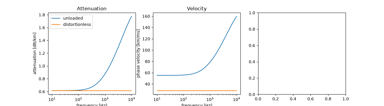
inductance needed for a distortionless line: 25 µH/m (42x the cable's)

<matplotlib.legend.Legend object at 0x111108a50>

A pulse down 20 km of line

The line is terminated in its characteristic impedance, so the received spectrum is the sent spectrum times \(e^{-\gamma\ell}\).

length, fs, n = 20e3, 1e6, 2**14
t = np.arange(n) / fs
pulse = np.exp(-0.5 * ((t - 1e-3) / 1e-4) ** 2)
w = 2 * np.pi * np.fft.rfftfreq(n, 1 / fs)
for L, name in ((L_cable, "unloaded"), (L_loaded, "distortionless")):
    gamma = np.concatenate(([np.sqrt(R * G)], propagation_constant(R, L, G, C, w[1:])))
    received = np.fft.irfft(np.fft.rfft(pulse) * np.exp(-gamma * length), n)
    axes[2].plot(t * 1e3, received / received.max(), label=name)
delay = length / transmission_line_velocity(L_loaded, C)
expected = np.exp(-np.sqrt(R * G) * length) * np.interp(t - delay, t, pulse)
print(f"distortionless delay {delay * 1e3:.3f} ms, amplitude {np.exp(-np.sqrt(R * G) * length):.3f}")
assert np.allclose(received, expected, atol=1e-6)
axes[2].plot(t * 1e3, pulse, ":", color="gray", label="sent")
axes[2].set(xlim=(0, 4), xlabel="time [ms]", ylabel="normalised voltage", title="Received pulse shape")
axes[2].legend()
fig.tight_layout()

plt.show()

distortionless delay 0.707 ms, amplitude 0.243