Smith’s chart (1939)

Phillip Hagar Smith, an engineer at Bell Labs, tired of evaluating the transmission-line equations with a slide rule. His 1939 chart plots the reflection coefficient \(\Gamma = (Z_L - Z_0)/(Z_L + Z_0)\) (reflection_coefficient()) in the unit disc, overlaid with circles of constant normalised resistance and arcs of constant reactance. Moving along a lossless line just rotates \(\Gamma\) around the centre, at constant standing-wave ratio (standing_wave_ratio()), so the input impedance (input_impedance()) can be read off the grid. This example uses the chart to design a single-stub match, drawn with plot_smith_chart().

import matplotlib.pyplot as plt
import numpy as np
from scipy.optimize import brentq

from engineeringkit.electrical_engineering import input_impedance, reflection_coefficient, standing_wave_ratio
from engineeringkit.electrical_engineering.visualizers import plot_smith_chart

Moving along the line

z0, zl = 50.0, 25.0 - 30.0j
gamma_l = reflection_coefficient(zl, z0)
print(f"load: Gamma = {abs(gamma_l):.3f} at {np.degrees(np.angle(gamma_l)):.1f} deg, VSWR = {standing_wave_ratio(gamma_l):.2f}")
bl = np.linspace(0, np.pi, 361)  # half a wavelength
locus = reflection_coefficient(input_impedance(zl, z0, bl), z0)
assert np.allclose(np.abs(locus), abs(gamma_l))  # a circle about the centre
assert np.isclose(input_impedance(zl, z0, np.pi), zl)  # half a wavelength repeats the load

load: Gamma = 0.483 at -108.0 deg, VSWR = 2.87

A shorted shunt stub

Move toward the generator until the input conductance is \(1/Z_0\) (the unit conductance circle), then cancel the remaining susceptance with a short-circuited stub in parallel.

def conductance_error(x):
    return (1 / input_impedance(zl, z0, x)).real - 1 / z0


error = conductance_error(bl)
k = np.flatnonzero(np.sign(error[:-1]) != np.sign(error[1:]))[0]  # first crossing of the circle
d = brentq(conductance_error, bl[k], bl[k + 1])
b = (1 / input_impedance(zl, z0, d)).imag
stub = brentq(lambda x: (1 / input_impedance(0, z0, x)).imag + b, 0.01, np.pi / 2 - 1e-9)
y_total = 1 / input_impedance(zl, z0, d) + 1 / input_impedance(0, z0, stub)
print(f"stub at {d / (2 * np.pi):.4f} wavelengths from the load, stub length {stub / (2 * np.pi):.4f} wavelengths")
print(f"matched input impedance {1 / y_total:.4f} ohm")
assert abs(reflection_coefficient(1 / y_total, z0)) < 1e-9

ax = plot_smith_chart(locus, label="along the line")
ax.plot(gamma_l.real, gamma_l.imag, "ks", label="load")
g_d = reflection_coefficient(input_impedance(zl, z0, d), z0)
ax.plot(g_d.real, g_d.imag, "C3o", label="stub position")
ax.plot(0, 0, "C2*", ms=12, label="matched")
ax.legend(loc="upper left", fontsize="small")
ax.set_title("Single-stub match on the Smith chart")

plt.show()

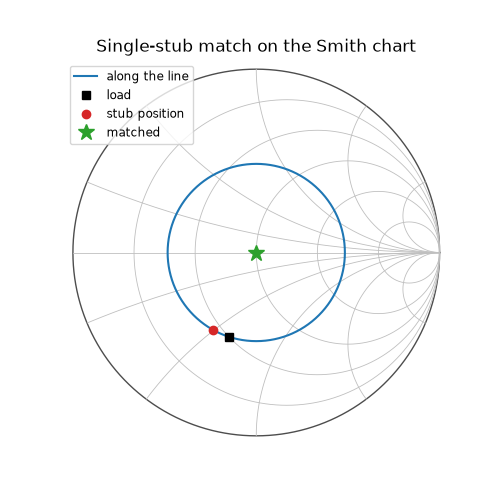
stub at 0.0151 wavelengths from the load, stub length 0.1171 wavelengths
matched input impedance 50.0000-0.0000j ohm