Moody’s diagram (1944)

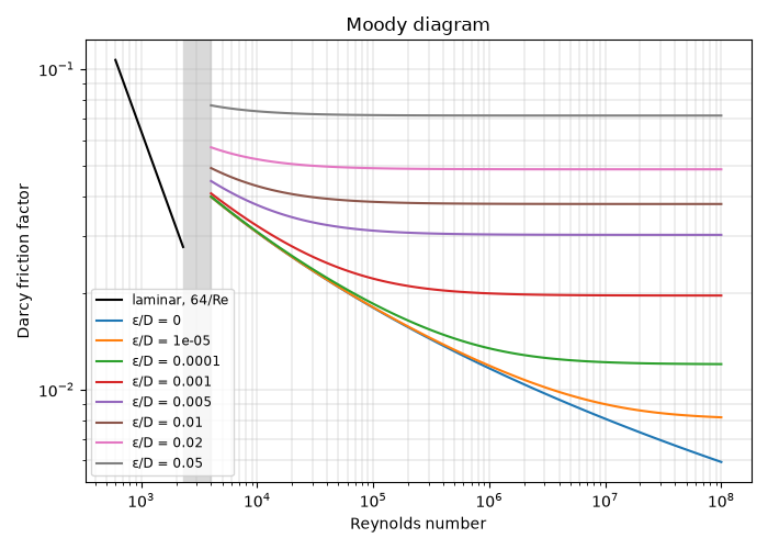
Lewis Moody, a Princeton professor of hydraulics, plotted Colebrook’s equation for the roughness of commercial pipes in 1944, together with the laminar line, on one log-log chart (plot_moody_diagram()). Engineers read friction factors from it for the next half-century. Moody also showed how to solve the three classic pipe problems with it: find the head loss, the flow, or the diameter. This example draws the chart and solves the third, which needs iteration even with colebrook_friction_factor() in hand.

import matplotlib.pyplot as plt
import numpy as np
from scipy import optimize

from engineeringkit.fluid_engineering import colebrook_friction_factor, darcy_head_loss, reynolds_number
from engineeringkit.fluid_engineering.visualizers import plot_moody_diagram

The chart

ax = plot_moody_diagram()
ax.figure.set_size_inches(7, 5)
ax.figure.tight_layout()

Reading the chart: water in commercial steel

Commercial steel has \(\varepsilon = 0.045\) mm. Water at 2 m/s in a 200 mm main has \(Re \approx 4\times10^5\).

rho, mu, eps = 998.0, 1.0e-3, 0.045e-3
Re = reynolds_number(rho, 2.0, 0.2, mu)
f = colebrook_friction_factor(Re, eps / 0.2)
ax.plot(Re, f, "k*", ms=12)
print(f"Re = {Re:.2e}, ε/D = {eps / 0.2:.2e}: f = {f:.4f}")

Re = 3.99e+05, ε/D = 2.25e-04: f = 0.0160

Moody’s third problem: choose the diameter

Which steel pipe carries 50 L/s over 1 km with no more than 10 m of head loss? The friction factor depends on the diameter through both \(Re\) and \(\varepsilon/D\), so the loss is solved for D.

Q, L, h_max = 0.050, 1000.0, 10.0


def loss(D):
    v = Q / (np.pi * D**2 / 4)
    return darcy_head_loss(colebrook_friction_factor(reynolds_number(rho, v, D, mu), eps / D), L, D, v)


D = optimize.brentq(lambda D: loss(D) - h_max, 0.05, 1.0)
print(f"smallest diameter: {1e3 * D:.1f} mm (loss at D: {loss(D):.3f} m)")

smallest diameter: 202.2 mm (loss at D: 10.000 m)

At fixed flow the loss falls roughly as \(D^{-5}\): a pipe 10% wider loses \(1.1^{-5} = 0.62\) of the head, a little less still because the friction factor falls too.

print(f"10% larger pipe: loss {loss(1.1 * D):.2f} m")
assert np.isclose(loss(D), h_max)
assert 0.55 < loss(1.1 * D) / h_max < 0.65
assert colebrook_friction_factor(1000.0, 0.01) == 64 / 1000

plt.show()

10% larger pipe: loss 6.22 m