Churchill and Bernstein: the cylinder in crossflow (1977)

Heat transfer from a cylinder in crossflow was long given by power laws fitted range by range (Hilpert’s of 1933 has five), each with its own constants. In 1977 Stuart Churchill and M. Bernstein, applying the method of blending asymptotes that Churchill had used for free convection, wrote a single expression from creeping flow past the drag crisis (churchill_bernstein_nusselt()). This example compares it with Hilpert’s table and calibrates a hot-wire anemometer with it.

import matplotlib.pyplot as plt
import numpy as np
from scipy.optimize import brentq

from engineeringkit.heat_transfer import churchill_bernstein_nusselt

Against Hilpert’s power laws

\(Nu = C\,Re^m Pr^{1/3}\) with the constants of Hilpert as tabulated by Incropera et al. (Table 7.2). Over five decades of Reynolds number the two stay within about 25% of each other, which is the scatter of the data they were both fitted to.

Pr = 0.71
hilpert = [
    (0.4, 4, 0.989, 0.330),
    (4, 40, 0.911, 0.385),
    (40, 4000, 0.683, 0.466),
    (4000, 40000, 0.193, 0.618),
    (40000, 400000, 0.027, 0.805),
]
fig, ax = plt.subplots(figsize=(6, 4))
worst = 0.0
for low, high, C, m in hilpert:
    Re = np.geomspace(low, high, 30)
    fit = C * Re**m * Pr ** (1 / 3)
    worst = max(worst, np.max(np.abs(churchill_bernstein_nusselt(Re, Pr) / fit - 1)))
    ax.loglog(Re, fit, "k:", lw=2)
Re_all = np.geomspace(0.4, 4e5, 300)
ax.loglog(Re_all, churchill_bernstein_nusselt(Re_all, Pr), label="Churchill-Bernstein")
ax.plot([], [], "k:", lw=2, label="Hilpert, five ranges")
ax.set(xlabel="Reynolds number", ylabel="average Nusselt number", title="Circular cylinder in crossflow, Pr = 0.71")
ax.legend()
fig.tight_layout()
print(f"largest gap to Hilpert's table: {worst:.0%}")
assert worst < 0.27

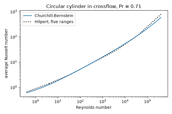
largest gap to Hilpert's table: 25%

A hot-wire anemometer

A 5 µm tungsten wire, 1 mm long, is held at 250 °C in air at 20 °C. The power it needs rises with the air speed, so measuring power measures speed. King (1914) showed it follows \(P = A + B\sqrt V\); the correlation reproduces that law at the wire’s tiny Reynolds numbers.

D, length, Tw, Ta = 5e-6, 1e-3, 523.15, 293.15
k, nu = 0.0336, 2.6e-5  # air at the 135 °C film temperature
speeds = np.linspace(0.5, 30, 40)
power = churchill_bernstein_nusselt(speeds * D / nu, Pr) * k / D * np.pi * D * length * (Tw - Ta)
B, A = np.polyfit(np.sqrt(speeds), power, 1)
king = A + B * np.sqrt(speeds)
print(f"King's law fit: P = {A * 1e3:.2f} mW + {B * 1e3:.2f} mW x sqrt(V [m/s]), Re up to {speeds[-1] * D / nu:.1f}")
assert np.max(np.abs(king / power - 1)) < 0.01

# Invert: read a speed from a measured power.
measured = 0.025
speed = brentq(lambda V: churchill_bernstein_nusselt(V * D / nu, Pr) * k * np.pi * length * (Tw - Ta) - measured, 0.01, 100)
print(f"a wire drawing {measured * 1e3:.0f} mW sits in air moving at {speed:.1f} m/s")
assert np.isclose(speed, ((measured - A) / B) ** 2, rtol=0.01)

fig, ax = plt.subplots(figsize=(6, 3.5))
ax.plot(speeds, power * 1e3, "o", label="Churchill-Bernstein")
ax.plot(speeds, king * 1e3, label="King's law fit")
ax.set(xlabel="air speed [m/s]", ylabel="wire power [mW]", title="Hot-wire calibration")
ax.legend()
fig.tight_layout()

plt.show()

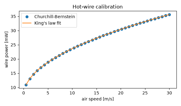
King's law fit: P = 7.27 mW + 5.18 mW x sqrt(V [m/s]), Re up to 5.8
a wire drawing 25 mW sits in air moving at 11.7 m/s