Kays and London: the effectiveness-NTU method (1955)

The log-mean temperature difference sizes an exchanger when all four end temperatures are known (log_mean_temperature_difference(), heat_exchanger_rate()). To rate a given exchanger, when only the inlets are known, it needs iteration. William Kays and Alexander London, testing compact exchangers for the US Navy at Stanford, organised everything around the effectiveness \(\varepsilon = \dot Q/\dot Q_{max}\) as a function of \(NTU = UA/C_{min}\) and \(C_r = C_{min}/C_{max}\) (exchanger_effectiveness_counterflow(), exchanger_effectiveness_parallel()), and published the charts in Compact Heat Exchangers (1955). This example rates an oil cooler both ways and marches the energy equations along it.

import matplotlib.pyplot as plt
import numpy as np
from scipy.integrate import solve_ivp

from engineeringkit.heat_transfer import (
    convection_resistance,
    exchanger_effectiveness_counterflow,
    exchanger_effectiveness_parallel,
    heat_exchanger_rate,
    log_mean_temperature_difference,
    overall_u,
    plane_wall_resistance,
)

An oil cooler

Oil (\(C_h = 2000\) W/K) enters at 400 K, water (\(C_c = 4000\) W/K) at 300 K. The tube wall is 1 mm of steel between film coefficients of 300 and 3000 W/(m² K); the area is 15 m².

C_h, C_c, Th_in, Tc_in, A = 2000.0, 4000.0, 400.0, 300.0, 15.0
UA = overall_u(convection_resistance(300.0, A), plane_wall_resistance(0.001, 45.0, A), convection_resistance(3000.0, A))
U = UA / A
C_min, C_max = min(C_h, C_c), max(C_h, C_c)
NTU, Cr = UA / C_min, C_min / C_max
eps = exchanger_effectiveness_counterflow(NTU, Cr)
Q = eps * C_min * (Th_in - Tc_in)
Th_out, Tc_out = Th_in - Q / C_h, Tc_in + Q / C_c
print(f"U = {U:.0f} W/(m² K), NTU = {NTU:.3f}, Cr = {Cr}, effectiveness {eps:.4f}")
print(f"duty {Q / 1e3:.2f} kW; oil leaves at {Th_out:.2f} K, water at {Tc_out:.2f} K")

U = 271 W/(m² K), NTU = 2.033, Cr = 0.5, effectiveness 0.7791
duty 155.82 kW; oil leaves at 322.09 K, water at 338.96 K

The LMTD method agrees

With the outlets now known, \(UA\,\Delta T_{lm}\) must return the same duty.

dt_lm = log_mean_temperature_difference(Th_in - Tc_out, Th_out - Tc_in)
Q_lmtd = heat_exchanger_rate(U, A, dt_lm)
print(f"LMTD {dt_lm:.3f} K gives {Q_lmtd / 1e3:.2f} kW")
assert np.isclose(Q_lmtd, Q, rtol=1e-10)

LMTD 38.321 K gives 155.82 kW

Marching along the exchanger

\(C_h\,\mathrm{d}T_h/\mathrm{d}a = -U(T_h - T_c)\) and, in counterflow, \(C_c\,\mathrm{d}T_c/\mathrm{d}a = -U(T_h - T_c)\) too. Integrating from the oil inlet with the computed water outlet must bring the water back to its inlet temperature.

def counterflow(a, T):
    q = U * (T[0] - T[1])
    return [-q / C_h, -q / C_c]


sol = solve_ivp(counterflow, (0, A), [Th_in, Tc_out], rtol=1e-11, atol=1e-9, dense_output=True)
print(f"water temperature at the far end {sol.y[1, -1]:.4f} K (inlet {Tc_in} K)")
assert np.isclose(sol.y[1, -1], Tc_in, atol=1e-5) and np.isclose(sol.y[0, -1], Th_out, atol=1e-5)

fig, axes = plt.subplots(1, 2, figsize=(10, 3.8))
a = np.linspace(0, A, 200)
axes[0].plot(a, sol.sol(a)[0], label="oil")
axes[0].plot(a, sol.sol(a)[1], label="water")
axes[0].set(xlabel="area from oil inlet [m²]", ylabel="temperature [K]", title="Counterflow oil cooler")
axes[0].legend()

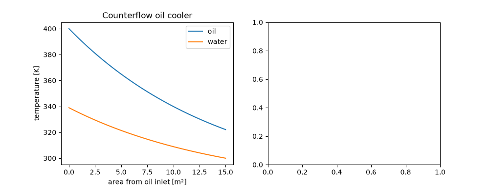
water temperature at the far end 300.0000 K (inlet 300.0 K)

<matplotlib.legend.Legend object at 0x11142fd90>

The effectiveness charts

Counterflow always beats parallel flow; parallel flow can never exceed \(1/(1 + C_r)\).

ntu = np.linspace(0, 5, 101)
for cr in [0.0, 0.5, 1.0]:
    counter = np.array([exchanger_effectiveness_counterflow(n, cr) for n in ntu])
    parallel = exchanger_effectiveness_parallel(ntu, cr)
    assert np.all(counter >= parallel - 1e-15) and np.all(parallel <= 1 / (1 + cr) + 1e-15)
    line = axes[1].plot(ntu, counter, label=f"counterflow Cr = {cr}")[0]
    axes[1].plot(ntu, parallel, "--", color=line.get_color())
axes[1].plot(NTU, eps, "ko")
axes[1].set(xlabel="NTU", ylabel="effectiveness", ylim=(0, 1), title="Solid: counterflow, dashed: parallel")
axes[1].legend()
fig.tight_layout()

plt.show()