Oppenheim’s radiation network (1956)

Between gray surfaces radiation is reflected back and forth, so every surface’s exchange depends on every other. Antoni Oppenheim, at Berkeley, replaced the bookkeeping by an electrical analogy: each surface’s blackbody emissive power drives current through a surface resistance \((1 - \varepsilon)/(\varepsilon A)\) to a node at its radiosity \(J\), and the radiosity nodes are joined by space resistances \(1/(A_iF_{ij})\). Insulated walls become floating nodes and radiation shields add resistances in series. The network needs view factors that obey reciprocity and summation (view_factor_reciprocity()); radiation_enclosure() solves it for any number of surfaces, and two_surface_radiation() (checked here on two facing plates) and radiation_shield_heat_flux() are its closed forms. This example models a furnace with a refractory wall and an insulated cryogenic line.

import matplotlib.pyplot as plt
import numpy as np

from engineeringkit.heat_transfer import (
    STEFAN_BOLTZMANN,
    radiation_enclosure,
    radiation_shield_heat_flux,
    two_surface_radiation,
    view_factor_coaxial_disks,
    view_factor_reciprocity,
)

A cylindrical furnace from reciprocity and summation

A furnace 1 m in diameter and 1 m long: a heated base (surface 1, 1500 K, \(\varepsilon = 0.8\)), a load on the top (surface 2, 500 K, \(\varepsilon = 0.6\)) and a refractory side wall (surface 3) that is insulated. Only \(F_{12}\) needs a formula; the other view factors follow from the two rules.

r, H = 0.5, 1.0
A = np.array([np.pi * r**2, np.pi * r**2, 2 * np.pi * r * H])
F12 = view_factor_coaxial_disks(r, r, H)
F13 = 1 - F12
F31 = view_factor_reciprocity(F13, A[0], A[2])
F = np.array([[0.0, F12, F13], [F12, 0.0, F13], [F31, F31, 1 - 2 * F31]])
print(f"F12 = {F12:.4f}, F13 = {F13:.4f}, F31 = {F31:.4f}, F33 = {F[2, 2]:.4f}")
assert np.allclose(F.sum(axis=1), 1) and np.allclose(A[:, None] * F, (A[:, None] * F).T)

furnace = radiation_enclosure([1500.0, 500.0, 0.0], [0.8, 0.6, 0.5], A, F, reradiating=[False, False, True])
print(f"heat to the load {furnace.heat_rate[0] / 1e3:.1f} kW; the refractory floats at {furnace.temperature[2]:.0f} K")

F12 = 0.1716, F13 = 0.8284, F31 = 0.2071, F33 = 0.5858
heat to the load 84.9 kW; the refractory floats at 1312 K

The network by hand

The refractory node sits on the two space resistances in series, \(1/(A_1F_{13}) + 1/(A_2F_{23})\), in parallel with the direct \(1/(A_1F_{12})\); the surface resistances add on each side.

R1, R2 = (1 - 0.8) / (0.8 * A[0]), (1 - 0.6) / (0.6 * A[1])
R12, R_via3 = 1 / (A[0] * F12), 1 / (A[0] * F13) + 1 / (A[1] * F13)
q_hand = STEFAN_BOLTZMANN * (1500.0**4 - 500.0**4) / (R1 + 1 / (1 / R12 + 1 / R_via3) + R2)
print(f"network by hand: {q_hand / 1e3:.1f} kW")
assert np.isclose(furnace.heat_rate[0], q_hand, rtol=1e-12)

# A water-cooled black side wall at 300 K would swallow most of the base's
# radiation instead of sending it on to the load.
cold = radiation_enclosure([1500.0, 500.0, 300.0], [0.8, 0.6, 1.0], A, F)
print(f"with a cold black side wall the load gets {cold.heat_rate[1] / -1e3:.1f} kW and the wall {cold.heat_rate[2] / -1e3:.1f} kW")
assert -cold.heat_rate[1] < furnace.heat_rate[0] and np.isclose(cold.heat_rate.sum(), 0.0, atol=1e-6)
assert np.isclose(
    two_surface_radiation(1500.0, 500.0, 0.8, 0.6, A[0], A[1], 1.0),
    radiation_enclosure([1500.0, 500.0], [0.8, 0.6], A[:2], [[0, 1], [1, 0]]).heat_rate[0],
)

network by hand: 84.9 kW
with a cold black side wall the load gets 17.1 kW and the wall 161.0 kW

Radiation shields on a cryogenic line

A liquid-nitrogen line (77 K) faces a 300 K jacket across a vacuum gap; both are stainless steel, \(\varepsilon = 0.3\). Each aluminium-foil shield (\(\varepsilon = 0.05\)) adds \(1/0.05 + 1/0.05 - 1 = 39\) to a series resistance that starts at 5.67.

counts = np.arange(0, 11)
flux = np.array([radiation_shield_heat_flux(300.0, 77.0, 0.3, 0.3, [0.05] * int(n)) for n in counts])
for n in (0, 1, 5, 10):
    print(f"{n:2d} shields: {flux[n]:.3f} W/m²")
resistance = 1 / 0.3 + 1 / 0.3 - 1
assert np.allclose(flux, flux[0] * resistance / (resistance + 39 * counts))

fig, axes = plt.subplots(1, 2, figsize=(10, 3.8))
furnace.plot(ax=axes[0])
axes[0].set_title("Furnace: net radiation leaving each surface")
axes[1].semilogy(counts, flux, "o-")
axes[1].set(xlabel="number of foil shields", ylabel="heat flux [W/m²]", title="Cryogenic line, 300 K to 77 K")
fig.tight_layout()

plt.show()

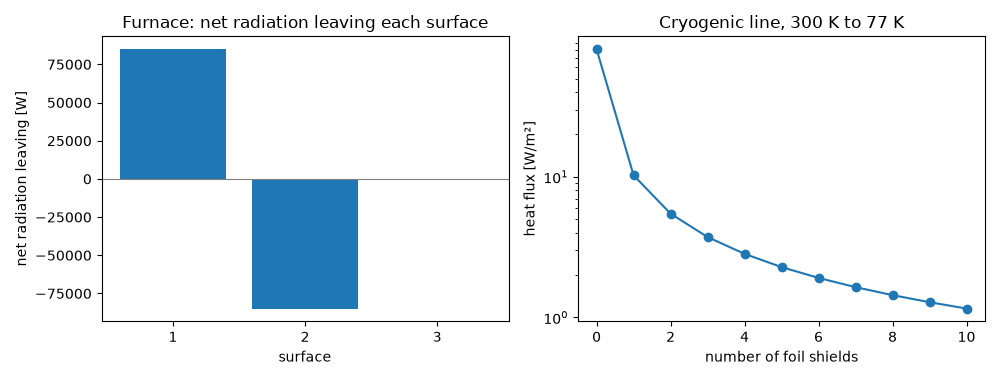
 0 shields: 80.701 W/m²
 1 shields: 10.238 W/m²
 5 shields: 2.279 W/m²
10 shields: 1.156 W/m²