The Larson-Miller parameter (1952)

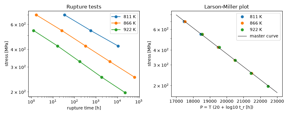
A boiler tube must last 100,000 hours, eleven years, but nobody can wait that long for a test. Frank Larson and James Miller (1952) observed that rupture times at different temperatures fall on one curve if plotted against \(P = T(C + \log_{10}t_r)\), with \(C \approx 20\) (larson_miller_parameter()). A short test at a higher temperature then stands in for a long life at a lower one (larson_miller_rupture_time()). The parameter follows from an Arrhenius rupture time \(t_r = t_0 e^{Q(\sigma)/RT}\): then \(C = -\log_{10}t_0\) and \(P = Q(\sigma)/(2.303R)\) depends on stress alone.

import matplotlib.pyplot as plt
import numpy as np

from engineeringkit.materials import larson_miller_parameter, larson_miller_rupture_time

HOUR = 3600.0

Rupture tests collapse onto one master curve

Stress-rupture tests on a low-alloy steel at three temperatures. Plotted against time they are three separate curves; against \(P\) they are one.

def master_stress(P):
    return 1e6 * 10 ** (2.9 - 1.1e-4 * (P - 17000))


temperatures = [811.0, 866.0, 922.0]
rng = np.random.default_rng(5)
tests = []
for T in temperatures:
    P = np.linspace(17500, 22500, 6)
    P = P[(P / T - 20 > -1) & (P / T - 20 < 5)]
    hours = 10 ** (P / T - 20) * rng.lognormal(0, 0.1, P.size)
    tests.append((T, hours * HOUR, master_stress(P)))

fig, (ax1, ax2) = plt.subplots(1, 2, figsize=(9.5, 3.8))
for T, t, s in tests:
    ax1.loglog(t / HOUR, s / 1e6, "o-", label=f"{T:.0f} K")
    P_test = larson_miller_parameter(T, t)
    ax2.semilogy(P_test, s / 1e6, "o", label=f"{T:.0f} K")
    assert np.allclose(master_stress(P_test), s, rtol=0.03)
P_line = np.linspace(17000, 23000, 50)
ax2.semilogy(P_line, master_stress(P_line) / 1e6, "k-", lw=0.8, label="master curve")
ax1.set(xlabel="rupture time [h]", ylabel="stress [MPa]", title="Rupture tests")
ax2.set(xlabel="P = T (20 + log10 t_r [h])", ylabel="stress [MPa]", title="Larson-Miller plot")
ax1.legend()
ax2.legend()
fig.tight_layout()

A short test for a long life

100,000 h at 811 K has \(P = 811 \times 25\). The same \(P\) is reached in 1000 h at \(811 \times 25/23 = 882\) K. The master curve gives the stress for that life.

design_T, design_life = 811.0, 1e5 * HOUR
P = larson_miller_parameter(design_T, design_life)
test_T = design_T * 25 / 23
print(f"P = {P:.0f}; 1000 h test at {test_T:.0f} K; allowable stress {master_stress(P) / 1e6:.0f} MPa")
assert np.isclose(larson_miller_rupture_time(P, test_T), 1000 * HOUR)
assert np.isclose(larson_miller_rupture_time(P, design_T), design_life)

plt.show()

P = 20275; 1000 h test at 882 K; allowable stress 347 MPa