Basquin’s S-N law (1910)

August Wöhler’s railway-axle tests of the 1860s showed that steel breaks under repeated stresses far below its static strength, and that below an endurance limit it may never break. Olin Basquin (1910) noticed that on log-log axes the finite-life part of Wöhler’s curves is a straight line, \(\sigma_a = \sigma_f'(2N)^b\) (basquin_cycles()). The example fits the line to scattered test results with power_law_fit() and recovers the constants that produced them.

import matplotlib.pyplot as plt
import numpy as np

from engineeringkit.materials import basquin_cycles
from engineeringkit.materials.utils import power_law_fit
from engineeringkit.materials.visualizers import plot_sn_curve

Simulated endurance tests

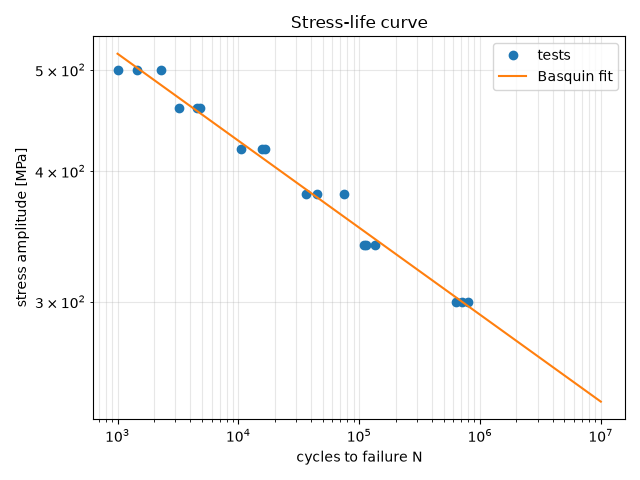
A steel with \(\sigma_f' = 1000\) MPa and \(b = -0.085\) is tested at six amplitudes, three specimens each. Fatigue lives scatter by a factor of a few, so each life gets a lognormal error.

sigma_f, b = 1000e6, -0.085
amplitudes = np.repeat(np.array([300, 340, 380, 420, 460, 500]) * 1e6, 3)
rng = np.random.default_rng(7)
lives = basquin_cycles(amplitudes, sigma_f, b) * rng.lognormal(0, 0.4, amplitudes.size)

A, p = power_law_fit(lives, amplitudes)
b_fit, sigma_f_fit = p, A / 2**p
print(f"fitted b = {b_fit:.4f} (true {b}), sigma_f' = {sigma_f_fit / 1e6:.0f} MPa (true {sigma_f / 1e6:.0f})")
assert abs(b_fit - b) < 0.01 and abs(sigma_f_fit / sigma_f - 1) < 0.15

fitted b = -0.0832 (true -0.085), sigma_f' = 975 MPa (true 1000)

The S-N diagram

One decade of life costs a fixed fraction of strength, \(10^{b}\), about 18% here. Wöhler’s endurance limit, the flat tail of a steel’s curve, is not part of Basquin’s law.

N = np.geomspace(1e3, 1e7, 50)
fitted = sigma_f_fit * (2 * N) ** b_fit
print(f"strength lost per decade of life: {100 * (1 - 10**b_fit):.1f}%")
assert np.allclose(basquin_cycles(fitted, sigma_f_fit, b_fit), N)

ax = plot_sn_curve(lives, amplitudes, style="o", label="tests")
plot_sn_curve(N, fitted, ax=ax, label="Basquin fit")
ax.set_title("Stress-life curve")
ax.figure.tight_layout()

plt.show()

strength lost per decade of life: 17.4%