Coffin and Manson: low-cycle fatigue (1954)

Nuclear plant and jet-engine parts heated and cooled a few thousand times fail by cycles of plastic strain, where Basquin’s stress-life law is useless because the stress hardly changes. Louis Coffin (1954) and Samson Manson (1953-1954) independently found that the plastic strain amplitude follows its own power law, \(\Delta\varepsilon_p/2 = \varepsilon_f'(2N)^c\) (coffin_manson_cycles()). Added to Basquin’s elastic line it gives the strain-life curve (strain_life_amplitude()) used for notched parts today.

import matplotlib.pyplot as plt
import numpy as np
from scipy.optimize import brentq

from engineeringkit.materials import basquin_cycles, coffin_manson_cycles, strain_life_amplitude

The strain-life curve

For a quenched and tempered steel, \(\sigma_f' = 1100\) MPa, \(b = -0.09\), \(\varepsilon_f' = 0.6\), \(c = -0.6\). Below the transition life plastic strain dominates; above it, elastic.

E, sf, b, ef, c = 200e9, 1100e6, -0.09, 0.6, -0.6
N = np.geomspace(10, 1e7, 300)
total, elastic, plastic = strain_life_amplitude(N, E, sf, b, ef, c)
Nt = 0.5 * (ef * E / sf) ** (1 / (b - c))
_, e_t, p_t = strain_life_amplitude(Nt, E, sf, b, ef, c)
print(f"transition life {Nt:.0f} cycles, where both strains are {e_t:.5f}")
assert np.isclose(e_t, p_t)

transition life 4950 cycles, where both strains are 0.00240

Life at a given strain

A part strained to \(\pm 0.8\%\) fails in about 1300 cycles. Its plastic part alone, put through Coffin-Manson, and its elastic part, put through Basquin, give the same life.

target = 0.008
life = brentq(lambda n: strain_life_amplitude(n, E, sf, b, ef, c)[0] - target, 1, 1e8)
_, e_life, p_life = strain_life_amplitude(life, E, sf, b, ef, c)
print(f"strain amplitude {target}: {life:.0f} cycles (plastic {p_life:.5f}, elastic {e_life:.5f})")
assert np.isclose(coffin_manson_cycles(p_life, ef, c), life) and np.isclose(basquin_cycles(e_life * E, sf, b), life)

fig, ax = plt.subplots(figsize=(6, 3.8))
ax.loglog(2 * N, total, label="total")
ax.loglog(2 * N, elastic, "--", label="elastic (Basquin)")
ax.loglog(2 * N, plastic, "--", label="plastic (Coffin-Manson)")
ax.axvline(2 * Nt, color="0.6", ls=":", label="transition")
ax.plot(2 * life, target, "ko")
ax.set(xlabel="reversals to failure 2N", ylabel="strain amplitude", title="Strain-life curve")
ax.legend()
fig.tight_layout()

plt.show()

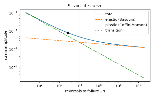
strain amplitude 0.008: 1327 cycles (plastic 0.00529, elastic 0.00271)