Neuber’s rule for notches that yield (1961)

A notch raises the elastic stress at its root by \(K_t\), but in a ductile part the root yields long before the nominal stress does, and \(K_t S\) overstates the stress and understates the strain. Heinz Neuber, at the Technical University of Munich, showed for a shear-loaded notch that the stress and strain concentration factors keep their geometric mean equal to \(K_t\) after yield, \(K_\sigma K_\varepsilon = K_t^2\), so

\[\sigma\varepsilon = \frac{(K_t S)^2}{E}\]

(neuber_notch_stress()). Intersected with the material’s stress-strain curve, the hyperbola gives the local strain that strain-life fatigue needs. The example also builds the fatigue notch factor from the notch sensitivity (peterson_notch_sensitivity(), fatigue_notch_factor()).

import matplotlib.pyplot as plt
import numpy as np

from engineeringkit.materials import (
    elliptical_hole_concentration,
    fatigue_notch_factor,
    neuber_notch_stress,
    peterson_notch_sensitivity,
    ramberg_osgood_strain,
)

Notch sensitivity

A hole in a wide plate has \(K_t = 3\) (Inglis). In fatigue a small hole hurts less: with Peterson’s material length \(\alpha = 0.25\) mm, a 1 mm radius gives \(q = 0.8\) and \(K_f = 2.6\).

Kt = elliptical_hole_concentration(1.0, 1.0)
q = peterson_notch_sensitivity(1e-3, 0.25e-3)
Kf = fatigue_notch_factor(Kt, q)
print(f"Kt = {Kt:.1f}, q = {q:.2f}, Kf = {Kf:.2f}")
assert np.isclose(Kf, 2.6)

Kt = 3.0, q = 0.80, Kf = 2.60

The Neuber hyperbola

A steel with \(E = 200\) GPa and a Ramberg-Osgood curve through a 0.2% offset yield of 400 MPa (\(n = 8\)) carries a nominal 250 MPa at the hole. The elastic answer, 750 MPa, is far above yield; Neuber gives a local stress near 440 MPa and a strain 1.7 times the elastic one.

E, sy, n, S = 200e9, 400e6, 8.0, 250e6
stress, strain = neuber_notch_stress(S, Kt, E, sy, n)
print(f"Neuber: sigma = {stress / 1e6:.0f} MPa, strain = {strain:.4f}; elastic: {Kt * S / 1e6:.0f} MPa, {Kt * S / E:.4f}")
assert np.isclose(stress * strain, (Kt * S) ** 2 / E) and stress < Kt * S and strain > Kt * S / E

curve_stress = np.linspace(0, 700e6, 300)
curve_strain = ramberg_osgood_strain(curve_stress, E, sy, n)
hyper_strain = np.linspace(0.0015, 0.012, 200)
fig, ax = plt.subplots(figsize=(6, 3.8))
ax.plot(curve_strain, curve_stress / 1e6, label="Ramberg-Osgood curve")
ax.plot(hyper_strain, (Kt * S) ** 2 / E / hyper_strain / 1e6, "--", label="Neuber hyperbola")
ax.plot([0, Kt * S / E], [0, Kt * S / 1e6], ":", color="0.4", label="elastic line")
ax.plot(strain, stress / 1e6, "ko", label="notch root")
ax.plot(Kt * S / E, Kt * S / 1e6, "kx", label="elastic estimate")
ax.set(xlim=(0, 0.012), ylim=(0, 800), xlabel="strain", ylabel="stress [MPa]", title="Neuber's rule at a hole")
ax.legend(fontsize=8)
fig.tight_layout()

plt.show()

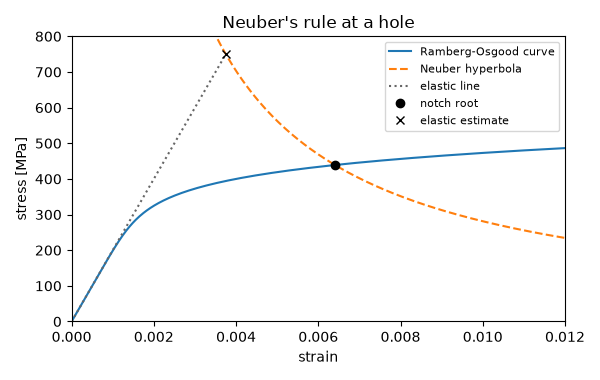
Neuber: sigma = 439 MPa, strain = 0.0064; elastic: 750 MPa, 0.0037