Aronhold and Kennedy’s theorem of three centres (1872-1886)

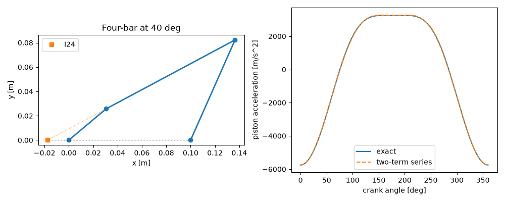
Every pair of links in a plane mechanism has an instant centre, a point where neither moves relative to the other. Siegfried Aronhold (1872) and, independently, Alexander Kennedy (1886) proved that the three instant centres of any three links lie on a straight line. For a four-bar linkage the centre \(I_{24}\) of crank and rocker lies where the line through the ground pivots meets the line of the coupler, and the speed ratio is the ratio of its distances from the pivots, \(\omega_4/\omega_2 = I_{12}I_{24}/I_{14}I_{24}\). The example checks this against the analytical velocity and acceleration analysis of fourbar_kinematics(), and checks slider_crank_kinematics() against its instant centre and against the engine designers’ two-term acceleration series.

import matplotlib.pyplot as plt
import numpy as np

from engineeringkit.mechanical_engineering import fourbar_kinematics, slider_crank_kinematics
from engineeringkit.mechanical_engineering.visualizers import plot_linkage

Four-bar: speed ratio from the instant centre

Ground pivots \(O_2 = (0, 0)\) and \(O_4 = (d, 0)\). \(I_{24}\) lies on the x axis (through \(I_{12} = O_2\) and \(I_{14} = O_4\)) and on the coupler line through \(A\) and \(B\).

a, b, c, d = 0.04, 0.12, 0.09, 0.10
omega2 = 30.0
theta2 = np.radians(np.arange(0, 360, 5))
motion = fourbar_kinematics(a, b, c, d, theta2, omega2)
A = a * np.exp(1j * theta2)
B = d + c * np.exp(1j * motion.theta4)
s = -A.imag / (B - A).imag  # A + s (B - A) on the x axis
x24 = (A + s * (B - A)).real
ratio = x24 / (x24 - d)  # signed distances from O2 and O4
print(f"largest |omega4/omega2 - IC ratio|: {np.max(np.abs(motion.omega4 / omega2 - ratio)):.1e}")
assert np.allclose(motion.omega4 / omega2, ratio)

largest |omega4/omega2 - IC ratio|: 3.3e-16

Slider-crank: velocity from the instant centre

The rod’s instant centre with the ground lies on the crank line, extended, and on the vertical through the slider, so the slider speed is the rod’s counter-clockwise angular velocity \(\omega_3\) times the height of that centre above the slider.

r, l, omega = 0.05, 0.18, 300.0
theta = np.radians(np.arange(5, 360, 10))
engine = slider_crank_kinematics(r, l, theta, omega)
height = np.tan(theta) * engine.position  # the crank line at x = slider position
omega3 = -engine.rod_angular_velocity  # rod angle beta is measured clockwise
assert np.allclose(engine.velocity, omega3 * height)
print(f"peak piston speed {engine.summary()['peak_velocity_m_s']:.2f} m/s at {omega * 60 / (2 * np.pi):.0f} rpm")

peak piston speed 15.57 m/s at 2865 rpm

Piston acceleration and its harmonics

\(\ddot x \approx -r\omega^2(\cos\theta + (r/l)\cos 2\theta)\); the exact value is largest at top dead centre, \(r\omega^2(1 + r/l)\).

full = slider_crank_kinematics(r, l, np.linspace(0, 2 * np.pi, 721), omega)
series = -r * omega**2 * (np.cos(full.theta) + r / l * np.cos(2 * full.theta))
assert np.isclose(full.acceleration[0], -r * omega**2 * (1 + r / l))
assert np.max(np.abs(full.acceleration - series)) < 0.03 * r * omega**2

fig, (ax1, ax2) = plt.subplots(1, 2, figsize=(10, 4))
k = 8
plot_linkage([[0, 0], [A[k].real, A[k].imag], [B[k].real, B[k].imag], [d, 0]], ax=ax1)
ax1.plot([min(0, x24[k]), max(d, x24[k])], [0, 0], "k:", lw=0.8)
ax1.plot([A[k].real, x24[k]], [A[k].imag, 0], "C1:", lw=0.8)
ax1.plot(x24[k], 0, "C1s", label="I24")
ax1.legend()
ax1.set(title=f"Four-bar at {np.degrees(theta2[k]):.0f} deg")
ax2.plot(np.degrees(full.theta), full.acceleration, label="exact")
ax2.plot(np.degrees(full.theta), series, "--", label="two-term series")
ax2.set(xlabel="crank angle [deg]", ylabel="piston acceleration [m/s^2]")
ax2.legend()
fig.tight_layout()

plt.show()