
Ctrl+K
engineeringkit logo engineeringkit logo
  • Subpackages
  • History
  • Examples
  • API
  • Subpackages
  • History
  • Examples
  • API

Section Navigation

  • Examples
    • Beams
    • Energy methods
    • Frames
    • Members
    • Plasticity
    • Stability
    • Stress
    • Trusses
  • Examples
    • Dynamics
    • Machine elements
    • Mechanisms
    • Rotordynamics
    • Transmission
    • Vibration
  • Examples
    • Cycles
    • Exergy
    • Laws
    • Properties
    • Psychrometrics
    • Refrigeration
  • Examples
    • Hydrostatics
    • Measurement
    • Networks
    • Open channels
    • Pipe flow
    • Pumps
    • Similarity
    • Transients
  • Examples
    • Conduction
    • Convection
    • Heat exchangers
    • Phase change
    • Radiation
    • Transient conduction
  • Examples
    • Airfoils
    • Standard atmosphere
    • Boundary layers
    • Circulation
    • Compressible flow
    • Forces and coefficients
    • Performance
    • Finite wings
  • Examples
    • AC circuits
    • DC circuits
    • Networks
    • Power
    • Transients
    • Transmission lines
  • Examples
    • Feedback
    • Frequency response
    • Optimal control and estimation
    • Root locus
    • Sampled-data control
    • Stability
    • State space
    • Time response
  • Examples
    • Filters
    • Fourier analysis
    • Sampling
    • Spectral analysis
    • Wavelets
  • Examples
    • Coding
    • Decibels
    • Detection
    • Information and capacity
    • Modulation
    • Multiplexing
    • Noise
    • Propagation
  • Examples
    • Composites
    • Creep
    • Elasticity
    • Fatigue
    • Fracture
    • Plasticity
    • Yield
  • Examples
    • Growth
    • Lifetimes
    • Maintenance
    • Risk
    • Structural reliability
    • Systems
  • Tutorials
    • A beam from load to fatigue life
    • A feedback loop in the time and frequency domains
    • A power plant from cycle to cooling tower
    • A radio link from antenna to bit errors
  • Exercises
    • Structural engineering exercises
    • Mechanical engineering exercises
    • Thermodynamics exercises
    • Fluid engineering exercises
    • Heat transfer exercises
    • Aerodynamics exercises
    • Electrical engineering exercises
    • Control systems exercises
    • Signal processing exercises
    • Communications exercises
    • Materials exercises
    • Reliability exercises
  • Installation and quickstart
  • Numerical methods and inspectable histories
  • Structural engineering: loads, signs and linear elasticity
  • Mechanical engineering: power, vibration and mechanism geometry
  • Thermodynamics: total versus specific quantities and cycle states
  • Fluid engineering: flow regimes and signed quantities
  • Heat transfer: absolute temperatures and resistance accounting
  • Aerodynamics: incompressible limits and compressible conservation
  • Electrical engineering: passive components and circuit responses
  • Control systems: matrix contracts and numerical stability
  • Signal processing: sampled energy, spectra and quantization
  • Communications: linear ratios, modulation phase and channel scope
  • Materials: elasticity, yield, fatigue, fracture and creep conventions
  • Reliability: distributions, independence and rate units
  • Examples
  • Examples
  • Mechanisms
  • Denavit and Hartenberg’s link parameters (1955)

Note

Go to the end to download the full example code or to run this example in your browser via JupyterLite.

Denavit and Hartenberg’s link parameters (1955)#

Jacques Denavit and Richard Hartenberg (1955) proposed a notation for any chain of links joined by lower pairs. Each link frame is placed so that going to the next takes only four numbers: a rotation \(\theta\) and a shift \(d\) along the joint axis \(z\), then a shift \(a\) and a twist \(\alpha\) along the common normal \(x\). The step is a single 4 by 4 homogeneous matrix (dh_transform()), and the pose of a robot’s hand is the product of one such matrix per joint (forward_kinematics()). The example checks the product against hand-derived trigonometry for a planar arm and a spatial articulated arm.

import matplotlib.pyplot as plt
import numpy as np

from engineeringkit.mechanical_engineering import dh_transform, forward_kinematics
from engineeringkit.mechanical_engineering.visualizers import plot_linkage

A planar three-link arm#

All joint axes are parallel (\(\alpha = 0\), \(d = 0\)), so the hand position is the sum of link vectors at cumulative angles.

lengths = np.array([0.4, 0.3, 0.15])
q = np.radians([30.0, 45.0, -60.0])
frames = forward_kinematics(np.column_stack((lengths, np.zeros(3), np.zeros(3), q)))
expected = np.array([np.sum(lengths * np.cos(np.cumsum(q))), np.sum(lengths * np.sin(np.cumsum(q)))])
print("planar hand position:", frames[-1][:2, 3].round(6).tolist(), "expected", expected.round(6).tolist())
assert np.allclose(frames[-1][:2, 3], expected)
assert np.isclose(np.arctan2(frames[-1][1, 0], frames[-1][0, 0]), np.sum(q))
planar hand position: [0.568945, 0.528601] expected [0.568945, 0.528601]

A spatial articulated arm#

A waist joint about the vertical (twist 90 degrees to the shoulder axis) carries a two-link planar arm, as in the PUMA’s first three joints. The hand lies at radius \(\rho = a_2\cos q_2 + a_3\cos(q_2 + q_3)\) from the waist axis, height \(d_1 + a_2\sin q_2 + a_3\sin(q_2 + q_3)\).

d1, a2, a3 = 0.5, 0.45, 0.4
for q1, q2, q3 in np.radians([[0, 30, -45], [60, 75, -120], [-135, 10, 30]]):
    table = [[0, np.pi / 2, d1, q1], [a2, 0, 0, q2], [a3, 0, 0, q3]]
    hand = forward_kinematics(table)[-1]
    rho = a2 * np.cos(q2) + a3 * np.cos(q2 + q3)
    expected = [rho * np.cos(q1), rho * np.sin(q1), d1 + a2 * np.sin(q2) + a3 * np.sin(q2 + q3)]
    print(f"q = {np.degrees([q1, q2, q3]).round(0).tolist()}: hand {hand[:3, 3].round(4).tolist()}")
    assert np.allclose(hand[:3, 3], expected)
    assert np.allclose(hand[:3, :3] @ hand[:3, :3].T, np.eye(3)) and np.isclose(np.linalg.det(hand[:3, :3]), 1)
q = [0.0, 30.0, -45.0]: hand [0.7761, 0.0, 0.6215]
q = [60.0, 75.0, -120.0]: hand [0.1997, 0.3458, 0.6518]
q = [-135.0, 10.0, 30.0]: hand [-0.53, -0.53, 0.8353]

The inverse step#

Each transform is a rigid motion, so its inverse is \([R^T,\ -R^T p]\) and the product of the two is the identity.

T = dh_transform(0.3, np.pi / 3, 0.1, 0.7)
inverse = np.eye(4)
inverse[:3, :3], inverse[:3, 3] = T[:3, :3].T, -T[:3, :3].T @ T[:3, 3]
assert np.allclose(T @ inverse, np.eye(4))

fig, ax = plt.subplots(figsize=(5.5, 4.5))
for angle in np.radians([0, 40, 80, 120]):
    pose = q + np.array([angle, -angle / 2, angle / 3])
    joints = forward_kinematics(np.column_stack((lengths, np.zeros(3), np.zeros(3), pose)))[:, :2, 3]
    plot_linkage(joints, ax=ax, alpha=0.8, label=f"first joint +{np.degrees(angle):.0f} deg")
ax.legend(fontsize=8)
ax.set(title="Planar arm poses from DH frames")
fig.tight_layout()

plt.show()
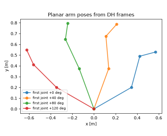
Planar arm poses from DH frames

Total running time of the script: (0 minutes 0.037 seconds)

Launch JupyterLite

Download Jupyter notebook: plot_04_denavit_hartenberg.ipynb

Download Python source code: plot_04_denavit_hartenberg.py

Download zipped: plot_04_denavit_hartenberg.zip

Gallery generated by Sphinx-Gallery

previous

Freudenstein’s equation for four-bar synthesis (1954)

next

Rotordynamics

On this page
  • A planar three-link arm
  • A spatial articulated arm
  • The inverse step
Show Source

Created using Sphinx 9.1.0.

Built with the PyData Sphinx Theme 0.22.0.