Arrhenius’s law and accelerated life testing (1889)

Svante Arrhenius (1889), measuring how fast acid inverts cane sugar, found that reaction rates grow with temperature as \(e^{-E_a/(k_B T)}\). Many failure mechanisms of electronics, such as diffusion, corrosion and intermetallic growth, are reactions, so a part’s life at temperature \(T\) scales as \(e^{E_a/(k_B T)}\). A test at 125 °C then stands in for years at 55 °C, through the acceleration factor (arrhenius_acceleration_factor()). Lives measured at several temperatures fix \(E_a\) (arrhenius_fit()).

import matplotlib.pyplot as plt
import numpy as np
from scipy.constants import eV, k, zero_Celsius

from engineeringkit.reliability import arrhenius_acceleration_factor, arrhenius_fit, weibull_mle

Three stress temperatures

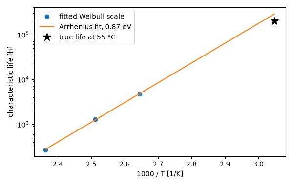
Capacitors with \(E_a\) = 0.8 eV and a Weibull life of shape 2 are tested, 15 units at each of 105, 125 and 150 °C. The Weibull scale fitted at each temperature is its characteristic life.

true_energy, use = 0.8 * eV, zero_Celsius + 55
eta_use = 2.0e5  # h at 55 degC
rng = np.random.default_rng(1889)
temperatures = zero_Celsius + np.array([105.0, 125.0, 150.0])
etas = []
for temperature in temperatures:
    eta = eta_use / arrhenius_acceleration_factor(true_energy, use, temperature)
    fit = weibull_mle(eta * rng.weibull(2.0, 15))
    etas.append(fit.eta)
    print(f"{temperature - zero_Celsius:5.0f} degC: true eta {eta:7.0f} h, fitted {fit.eta:7.0f} h")
etas = np.array(etas)

energy, constant = arrhenius_fit(temperatures, etas)
predicted = constant * np.exp(energy / (k * use))
print(f"fitted Ea = {energy / eV:.2f} eV; predicted eta at 55 degC = {predicted:.3g} h (true {eta_use:.3g} h)")
print(f"acceleration factor 55 -> 125 degC: {arrhenius_acceleration_factor(energy, use, temperatures[1]):.0f}")

  105 degC: true eta    4748 h, fitted    4672 h
  125 degC: true eta    1383 h, fitted    1304 h
  150 degC: true eta     349 h, fitted     270 h
fitted Ea = 0.87 eV; predicted eta at 55 degC = 2.86e+05 h (true 2e+05 h)
acceleration factor 55 -> 125 degC: 230

The Arrhenius plot

\(\ln L\) against \(1/T\) is a straight line of slope \(E_a/k_B\); extrapolating it to the use temperature is the whole prediction, and its uncertainty grows with the distance extrapolated.

fig, ax = plt.subplots(figsize=(6, 3.8))
inverse = np.linspace(1 / temperatures[-1], 1 / use, 50)
ax.semilogy(1000 / temperatures, etas, "o", label="fitted Weibull scale")
ax.semilogy(1000 * inverse, constant * np.exp(energy / (k / inverse)), "-", label=f"Arrhenius fit, {energy / eV:.2f} eV")
ax.semilogy(1000 / use, eta_use, "k*", ms=12, label="true life at 55 °C")
ax.set(xlabel="1000 / T [1/K]", ylabel="characteristic life [h]")
ax.legend()
fig.tight_layout()

assert abs(energy / eV - 0.8) < 0.1
assert 0.4 < predicted / eta_use < 2.5
assert np.isclose(arrhenius_acceleration_factor(true_energy, use, use), 1.0)

plt.show()