Eyring’s activated complex (1935)

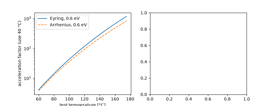
Henry Eyring (1935) derived reaction rates from statistical mechanics: reactants pass through an activated complex, and the rate is \((k_B T/h)\,e^{-\Delta G^\ddagger/(k_B T)}\). The prefactor \(T\) is absent from Arrhenius’s empirical law. For life testing it means \(L \propto T^{-1}e^{E_a/(k_B T)}\), and an acceleration factor \(T_t/T_u\) times the Arrhenius one (eyring_acceleration_factor()). The model extends naturally to non-thermal stresses such as voltage, here represented by the inverse power law (inverse_power_law_acceleration_factor()).

import matplotlib.pyplot as plt
import numpy as np
from scipy.constants import eV, k, zero_Celsius

from engineeringkit.reliability import (
    arrhenius_acceleration_factor,
    arrhenius_fit,
    eyring_acceleration_factor,
    inverse_power_law_acceleration_factor,
)

Eyring versus Arrhenius on the same data

Lives that follow Eyring’s law exactly with \(E_a\) = 0.6 eV are fitted with Arrhenius’s law. The fit absorbs the \(1/T\) prefactor into a slightly larger activation energy, about \(k_B \bar T\).

energy = 0.6 * eV
temperatures = zero_Celsius + np.array([85.0, 105.0, 125.0, 150.0])
lives = 1e-2 / temperatures * np.exp(energy / (k * temperatures))
arrhenius_energy, _ = arrhenius_fit(temperatures, lives)
print(f"Eyring Ea = {energy / eV:.3f} eV; Arrhenius fit to the same lives: {arrhenius_energy / eV:.3f} eV")
difference = (arrhenius_energy - energy) / eV * 1000
print(f"difference {difference:.1f} meV; k_B T at the mean test temperature {k * temperatures.mean() / eV * 1000:.1f} meV")

use = zero_Celsius + 40.0
test = np.linspace(zero_Celsius + 60, zero_Celsius + 175, 100)
fig, axes = plt.subplots(1, 2, figsize=(9, 3.5))
axes[0].semilogy(test - zero_Celsius, eyring_acceleration_factor(energy, use, test), label="Eyring, 0.6 eV")
axes[0].semilogy(test - zero_Celsius, arrhenius_acceleration_factor(energy, use, test), "--", label="Arrhenius, 0.6 eV")
axes[0].set(xlabel="test temperature [°C]", ylabel="acceleration factor (use 40 °C)")
axes[0].legend()

Eyring Ea = 0.600 eV; Arrhenius fit to the same lives: 0.634 eV
difference 33.5 meV; k_B T at the mean test temperature 33.6 meV

<matplotlib.legend.Legend object at 0x7fa1ee1909e0>

Combined temperature and voltage stress

A generalised Eyring model multiplies a thermal factor by a stress factor. For a dielectric with life \(\propto V^{-n}\), \(n = 3\), testing at twice the rated voltage and 125 °C multiplies the thermal acceleration by \(2^3\).

voltage = np.linspace(1, 3, 50)
for n in (2, 3, 5):
    axes[1].semilogy(voltage, inverse_power_law_acceleration_factor(1.0, voltage, n), label=f"n = {n}")
axes[1].set(xlabel="test voltage / rated voltage", ylabel="voltage acceleration factor")
axes[1].legend()
fig.tight_layout()

combined = eyring_acceleration_factor(energy, use, zero_Celsius + 125) * inverse_power_law_acceleration_factor(1.0, 2.0, 3)
print(f"combined acceleration at 125 degC and twice rated voltage: {combined:.0f}")

assert 0 < (arrhenius_energy - energy) / k < 1.2 * temperatures.mean()
assert np.isclose(eyring_acceleration_factor(energy, use, test[-1]), arrhenius_acceleration_factor(energy, use, test[-1]) * test[-1] / use)
assert np.isclose(inverse_power_law_acceleration_factor(1.0, 2.0, 3), 8.0)

plt.show()

combined acceleration at 125 degC and twice rated voltage: 1172