Johnson’s median ranks (1951)

Where should the \(i\)-th of \(n\) failures be plotted? The population fraction failed at the \(i\)-th smallest life is itself random, with a \(\mathrm{Beta}(i, n - i + 1)\) distribution. Leonard Johnson (1951), working on bearing fatigue at General Motors, proposed its median, the median rank, as the plotting position, and Benard’s \((i - 0.3)/(n + 0.4)\) approximates it closely (median_ranks()). For censored data Johnson’s adjusted order numbers (adjusted_ranks()) let units removed early still move the later ranks. A least-squares line on Weibull axes then gives \(\beta\) and \(\eta\) (weibull_rank_regression()).

import matplotlib.pyplot as plt
import numpy as np
from scipy import stats

from engineeringkit.reliability import adjusted_ranks, median_ranks, weibull_rank_regression

The median rank is the median of a beta distribution

Simulate many samples of ten lives from any continuous distribution: the fraction failed at the third failure, \(F(t_{(3)})\), is uniform order statistic number three of ten.

n = 10
rng = np.random.default_rng(1951)
u = np.sort(rng.random((100_000, n)), axis=1)
simulated = np.median(u, axis=0)
exact, benard = median_ranks(n), median_ranks(n, method="benard")
for i in (1, 3, 5, 10):
    print(f"i = {i:2d}: simulated {simulated[i - 1]:.4f}, beta median {exact[i - 1]:.4f}, Benard {benard[i - 1]:.4f}, i/n {i / n:.2f}")

fig, axes = plt.subplots(1, 2, figsize=(9, 3.5))
x = np.linspace(0, 1, 300)
for i in (1, 3, 5, 10):
    axes[0].plot(x, stats.beta.pdf(x, i, n - i + 1), label=f"i = {i}")
    axes[0].axvline(exact[i - 1], ls=":", color="gray")
axes[0].set(xlabel="fraction failed F", ylabel="density", title="Distribution of F at the i-th failure", ylim=(0, 10))
axes[0].legend()

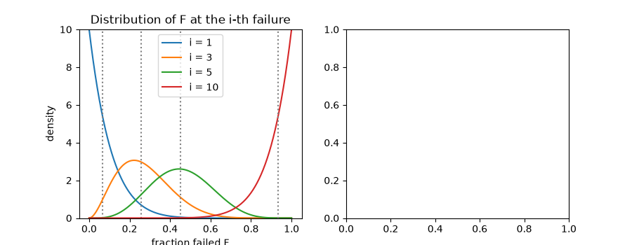
i =  1: simulated 0.0667, beta median 0.0670, Benard 0.0673, i/n 0.10
i =  3: simulated 0.2582, beta median 0.2586, Benard 0.2596, i/n 0.30
i =  5: simulated 0.4518, beta median 0.4517, Benard 0.4519, i/n 0.50
i = 10: simulated 0.9330, beta median 0.9330, Benard 0.9327, i/n 1.00

<matplotlib.legend.Legend object at 0x7f1af869e5a0>

Censored bearings on Weibull paper

Twelve bearings (\(\eta\) = 1000 h, \(\beta\) = 2) are tested; four are removed for other reasons before they fail. Their removal raises the order numbers of the failures that follow.

times = np.array([180, 310, 390, 450, 520, 610, 700, 760, 830, 980, 1150, 1400.0])
failed = np.array([1, 1, 0, 1, 1, 0, 1, 1, 0, 1, 0, 1])
failure_times, order = adjusted_ranks(times, failed)
print("adjusted order numbers:", np.round(order, 2))
fit = weibull_rank_regression(times, failed)
print(f"rank regression: beta = {fit.beta:.2f}, eta = {fit.eta:.0f} h, B10 life = {fit.b_life(0.1):.0f} h")
fit.plot(ax=axes[1])
fig.tight_layout()

assert np.allclose(simulated, exact, atol=0.003)
assert np.max(np.abs(benard - exact)) < 0.003
assert np.isclose(order[0], 1) and np.all(np.diff(order) >= 1) and order[-1] < times.size + 1
assert np.allclose(median_ranks(times.size, order), fit.median_ranks)

plt.show()

adjusted order numbers: [ 1.    2.    3.1   4.2   5.46  6.71  8.29 10.64]
rank regression: beta = 1.69, eta = 968 h, B10 life = 256 h