Raiffa and Schlaifer’s conjugate prior for a failure rate (1961)

Howard Raiffa and Robert Schlaifer (1961) named and catalogued conjugate priors, families that a likelihood maps into themselves. For failures that arrive as a Poisson process the conjugate family is the gamma distribution: a \(\mathrm{Gamma}(a, b)\) prior on the rate \(\lambda\) and \(r\) failures in time \(T\) give a \(\mathrm{Gamma}(a + r, b + T)\) posterior (bayesian_failure_rate()). Handbook or similar-part data set the prior (gamma_prior_from_bounds()), so a short test of a new part is not read in isolation.

import matplotlib.pyplot as plt
import numpy as np
from scipy import stats

from engineeringkit.reliability import bayesian_failure_rate, gamma_prior_from_bounds, mtbf_confidence_bounds

A prior from engineering judgement

Similar valves fail at about 2 per million hours, and almost certainly (95%) below 8 per million hours. Rates are per hour here.

shape, rate = gamma_prior_from_bounds(2e-6, 8e-6, 0.95)
print(f"prior: Gamma(a = {shape:.2f}, b = {rate:.3g} h), mean {shape / rate * 1e6:.2f} per 10^6 h")

prior: Gamma(a = 1.11, b = 4.01e+05 h), mean 2.77 per 10^6 h

Update on a short test, and on a long one

The new valve sees 1 failure in 200 000 unit-hours, then 6 failures in 3 million unit-hours.

fig, ax = plt.subplots(figsize=(6, 3.8))
lam = np.linspace(0, 1.2e-5, 400)
ax.plot(lam * 1e6, stats.gamma.pdf(lam, shape, scale=1 / rate) / 1e6, "--", label="prior")
for failures, hours in ((1, 2e5), (6, 3e6)):
    posterior = bayesian_failure_rate(shape, rate, failures, hours)
    classical = failures / hours
    print(
        f"{failures} failures in {hours:.0e} h: classical {classical * 1e6:.2f}, posterior mean {posterior.mean * 1e6:.2f}, "
        f"90% upper bound {posterior.upper_bound(0.9) * 1e6:.2f} per 10^6 h"
    )
    ax.plot(lam * 1e6, stats.gamma.pdf(lam, posterior.shape, scale=1 / posterior.rate) / 1e6, label=f"after {failures} in {hours:.0e} h")
ax.set(xlabel="failure rate [per $10^6$ h]", ylabel="density", title="Gamma prior and posteriors")
ax.legend()
fig.tight_layout()

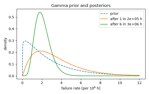
1 failures in 2e+05 h: classical 5.00, posterior mean 3.51, 90% upper bound 6.75 per 10^6 h
6 failures in 3e+06 h: classical 2.00, posterior mean 2.09, 90% upper bound 3.14 per 10^6 h

The posterior mean always lies between the prior mean and \(r/T\), and moves toward the data as test time accumulates. With a vague prior (\(a, b \to 0\)) the 90% upper bound is the classical chi-square bound with \(2r\) degrees of freedom; a prior with \(a = 1\) and \(b \to 0\) gives the time-terminated bound with \(2r + 2\).

vague = bayesian_failure_rate(1e-9, 1e-9, 6, 3e6)
flat = bayesian_failure_rate(1.0, 1e-9, 6, 3e6)
failure_terminated, _ = mtbf_confidence_bounds(3e6, 6, confidence=0.8)
time_terminated, _ = mtbf_confidence_bounds(3e6, 6, confidence=0.8, time_terminated=True)
print(f"a -> 0: 90% upper bound {vague.upper_bound(0.9) * 1e6:.3f}, chi-square 2r: {1e6 / failure_terminated:.3f} per 10^6 h")
print(f"a = 1:  90% upper bound {flat.upper_bound(0.9) * 1e6:.3f}, chi-square 2r + 2: {1e6 / time_terminated:.3f} per 10^6 h")

short, long = bayesian_failure_rate(shape, rate, 1, 2e5), bayesian_failure_rate(shape, rate, 6, 3e6)
assert np.isclose(stats.gamma.median(shape, scale=1 / rate), 2e-6)
assert min(shape / rate, 1 / 2e5) < short.mean < max(shape / rate, 1 / 2e5)
assert abs(long.mean - 6 / 3e6) < abs(short.mean - 1 / 2e5)
assert np.isclose(vague.upper_bound(0.9), 1 / failure_terminated, rtol=1e-6)
assert np.isclose(flat.upper_bound(0.9), 1 / time_terminated, rtol=1e-6)

plt.show()

a -> 0: 90% upper bound 3.092, chi-square 2r: 3.092 per 10^6 h
a = 1:  90% upper bound 3.511, chi-square 2r + 2: 3.511 per 10^6 h