Epstein and Sobel’s exponential life testing (1953)

How long must a test run, and with how many units, to demonstrate an MTBF? Epstein and Sobel (1953) showed that for exponential lives the total time on test \(T\), summed over failed and surviving units, carries all the information: \(\hat\theta = T/r\) after \(r\) failures, and \(2T/\theta\) is chi-square with \(2r\) degrees of freedom. That gives exact confidence bounds (mtbf_confidence_bounds()). The example stops a test of 12 units at the fourth failure, many times over, and checks that the 90% bounds catch the true MTBF 90% of the time.

import matplotlib.pyplot as plt
import numpy as np

from engineeringkit.reliability import exponential_mttf, exponential_reliability, failure_rate_from_mtbf, mtbf_confidence_bounds

One test

Components with a failure rate of \(2\times10^{-4}\) per hour (time unit: hours). Twelve go on test; the test stops at the fourth failure, so eight units are still running.

lam = 2e-4
theta = exponential_mttf(lam)
n, r = 12, 4
rng = np.random.default_rng(1953)
life = np.sort(rng.exponential(theta, n))
total = life[:r].sum() + (n - r) * life[r - 1]
low, high = mtbf_confidence_bounds(total, r, confidence=0.9)
print(f"test stopped at {life[r - 1]:.0f} h, total time on test {total:.0f} h")
print(f"MTBF estimate {total / r:.0f} h, 90% bounds [{low:.0f}, {high:.0f}] h (true {theta:.0f} h)")
print(f"estimated failure rate {failure_rate_from_mtbf(total / r):.2e}/h")

test stopped at 2502 h, total time on test 23477 h
MTBF estimate 5869 h, 90% bounds [3028, 17183] h (true 5000 h)
estimated failure rate 1.70e-04/h

Repeat the test 300 times

tests = 300
bounds = []
for _ in range(tests):
    life = np.sort(rng.exponential(theta, n))
    bounds.append(mtbf_confidence_bounds(life[:r].sum() + (n - r) * life[r - 1], r, 0.9))
bounds = np.array(bounds)
covered = (bounds[:, 0] <= theta) & (theta <= bounds[:, 1])
print(f"intervals containing the true MTBF: {covered.mean():.1%}")

fig, axes = plt.subplots(1, 2, figsize=(9.5, 3.8))
show = np.arange(60)
axes[0].vlines(show, bounds[show, 0], bounds[show, 1], colors=np.where(covered[show], "C0", "C3"))
axes[0].axhline(theta, color="k", lw=1)
axes[0].set(yscale="log", xlabel="test", ylabel="MTBF [h]", title="90% bounds, 60 of the tests")
t = np.linspace(0, 3 * theta, 200)
axes[1].plot(t, exponential_reliability(t, lam), label="true")
axes[1].fill_between(t, exponential_reliability(t, 1 / low), exponential_reliability(t, 1 / high), alpha=0.3, label="90% band, first test")
axes[1].set(xlabel="time [h]", ylabel="reliability")
axes[1].legend()
fig.tight_layout()

assert abs(covered.mean() - 0.9) < 0.05

plt.show()

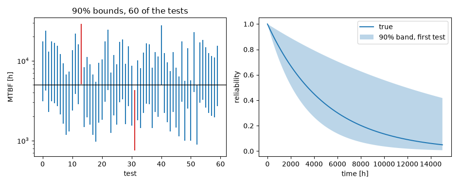
intervals containing the true MTBF: 90.0%