Weibull’s distribution and the Weibull plot (1951)

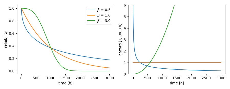
Waloddi Weibull (1951) proposed \(R(t) = e^{-(t/\eta)^\beta}\) (weibull_reliability()) for anything from the strength of steel to the life of bearings. The shape \(\beta\) sets the hazard (weibull_hazard()): falling for \(\beta < 1\), constant at 1, rising above. Because \(\ln(-\ln R) = \beta \ln t - \beta \ln \eta\), failure data plotted on those axes fall on a line whose slope is \(\beta\). The example fits a small life test that way and compares the mean life with weibull_mttf().

import matplotlib.pyplot as plt
import numpy as np

from engineeringkit.reliability import weibull_cdf, weibull_hazard, weibull_mttf, weibull_reliability

Three shapes, three hazards

t = np.linspace(0.01, 3000, 400)
eta = 1000.0
fig, axes = plt.subplots(1, 2, figsize=(9, 3.5))
for beta in (0.5, 1.0, 3.0):
    axes[0].plot(t, weibull_reliability(t, eta, beta), label=rf"$\beta$ = {beta}")
    axes[1].plot(t, weibull_hazard(t, eta, beta) * 1e3, label=rf"$\beta$ = {beta}")
axes[0].set(xlabel="time [h]", ylabel="reliability")
axes[1].set(xlabel="time [h]", ylabel="hazard [1/1000 h]", ylim=(0, 6))
axes[0].legend()
fig.tight_layout()

Fit a life test on Weibull paper

Thirty bearings with \(\eta\) = 1000 h and \(\beta\) = 2.5 run to failure. Bernard’s median ranks \((i - 0.3)/(n + 0.4)\) estimate \(F\) at the ordered failure times.

rng = np.random.default_rng(1951)
true_eta, true_beta, n = 1000.0, 2.5, 30
life = np.sort(true_eta * rng.weibull(true_beta, n))
F = (np.arange(1, n + 1) - 0.3) / (n + 0.4)
slope, intercept = np.polyfit(np.log(life), np.log(-np.log(1 - F)), 1)
beta_hat, eta_hat = slope, np.exp(-intercept / slope)
print(f"fitted beta = {beta_hat:.2f}, eta = {eta_hat:.0f} h; MTTF = {weibull_mttf(eta_hat, beta_hat):.0f} h")

fig, ax = plt.subplots(figsize=(5.5, 4))
ax.plot(np.log(life), np.log(-np.log(1 - F)), "o", label="median ranks")
x = np.linspace(np.log(life[0]), np.log(life[-1]))
ax.plot(x, np.log(-np.log(1 - weibull_cdf(np.exp(x), eta_hat, beta_hat))), label=rf"fit: $\beta$ = {beta_hat:.2f}")
ax.set(xlabel="ln(time)", ylabel="ln(-ln(1 - F))", title="Weibull plot")
ax.legend()
fig.tight_layout()

assert abs(beta_hat - true_beta) < 0.6 and abs(eta_hat / true_eta - 1) < 0.15
assert np.isclose(weibull_mttf(eta, 1.0), eta)

plt.show()

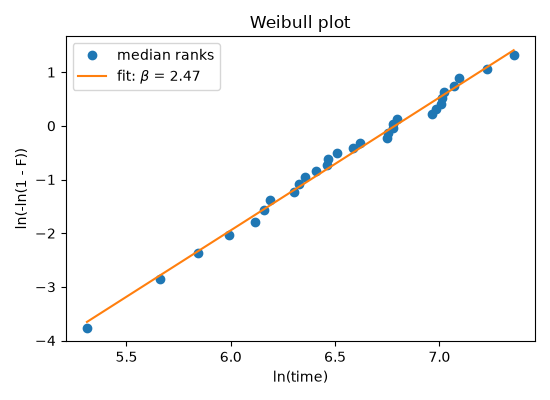
fitted beta = 2.47, eta = 886 h; MTTF = 786 h