Barlow and Proschan’s age replacement (1965)

Should a part be replaced on a schedule, before it fails? Richard Barlow and Frank Proschan answered with renewal theory. Replace at age \(T\) or at failure, whichever comes first. Each cycle then costs \(c_p R(T) + c_f F(T)\) and lasts \(\int_0^T R\,dt\) on average, so the long-run cost rate is their ratio (age_replacement_cost_rate()). A finite best age exists only if the hazard rises (Weibull \(\beta > 1\)) and a failure costs more than a planned replacement. With a constant hazard a new part is no better than the old one, so planned replacement only adds cost (renewal_interval_cost_rate()).

import matplotlib.pyplot as plt
import numpy as np
from scipy.optimize import minimize_scalar

from engineeringkit.reliability import (
    age_replacement_cost_rate,
    renewal_interval_cost_rate,
    weibull_hazard,
    weibull_mttf,
    weibull_reliability,
)

The optimum replacement age

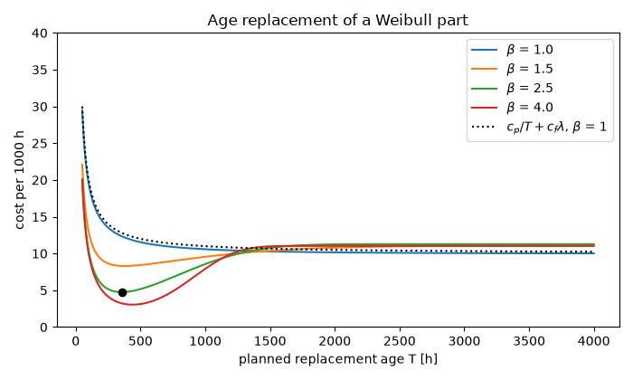
A wear-out bearing, Weibull \(\eta = 1000\) h, \(\beta = 2.5\). A planned change costs 1 unit, a failure in service 10. At the optimum the cost rate equals \((c_f - c_p)\,h(T^*)\).

eta, beta, cp, cf = 1000.0, 2.5, 1.0, 10.0
best = minimize_scalar(
    lambda T: age_replacement_cost_rate(T, cp, cf, eta, beta), bounds=(10, 5000), method="bounded", options={"xatol": 1e-6}
)
T_star, C_star = best.x, best.fun
run_to_failure = cf / weibull_mttf(eta, beta)
print(f"replace at {T_star:.0f} h: {C_star * 1000:.3f} per 1000 h; run to failure: {run_to_failure * 1000:.3f} per 1000 h")
print(f"saving {1 - C_star / run_to_failure:.0%}; {1 - weibull_reliability(T_star, eta, beta):.1%} still fail before T*")
assert np.isclose(C_star, (cf - cp) * weibull_hazard(T_star, eta, beta), rtol=1e-4)

replace at 355 h: 4.751 per 1000 h; run to failure: 11.271 per 1000 h
saving 58%; 7.2% still fail before T*

Check by simulating the renewal process

rng = np.random.default_rng(1965)
lives = eta * rng.weibull(beta, size=400_000)
failed = lives < T_star
simulated = (cf * failed.sum() + cp * (~failed).sum()) / np.minimum(lives, T_star).sum()
print(f"simulated cost rate {simulated * 1000:.3f} per 1000 h")
assert np.isclose(simulated, C_star, rtol=0.01)

simulated cost rate 4.743 per 1000 h

When planned replacement does not pay

With \(\beta = 1\) the cost rate falls monotonically to the run-to-failure value; the constant-hazard baseline \(c_p/T + c_f\lambda\) lies above it for every interval.

T = np.linspace(50, 4000, 400)
fig, ax = plt.subplots(figsize=(7, 4.2))
for shape in (1.0, 1.5, 2.5, 4.0):
    ax.plot(T, 1000 * age_replacement_cost_rate(T, cp, cf, eta, shape), label=rf"$\beta$ = {shape}")
constant = age_replacement_cost_rate(T, cp, cf, eta, 1.0)
baseline = renewal_interval_cost_rate(cp, cf, 1 / eta, T)
ax.plot(T, 1000 * baseline, "k:", label=r"$c_p/T + c_f\lambda$, $\beta$ = 1")
ax.plot(T_star, 1000 * C_star, "ko")
ax.set(xlabel="planned replacement age T [h]", ylabel="cost per 1000 h", ylim=(0, 40), title="Age replacement of a Weibull part")
ax.legend()
fig.tight_layout()

assert np.all(np.diff(constant) < 0) and np.all(baseline > constant)
assert C_star < run_to_failure

plt.show()