Markov models of repairable systems (1965)

A repairable unit fails and is mended over and over, so the question is not whether it survives but what fraction of time it is up. If failures and repairs both happen at constant rates, the unit is a continuous-time Markov chain. Barlow and Proschan’s 1965 monograph put such models at the centre of reliability theory. For one unit the up-probability decays from one to the steady state \(\mu/(\lambda + \mu) = \mathrm{MTBF}/(\mathrm{MTBF} + \mathrm{MTTR})\) with time constant \(1/(\lambda + \mu)\) (markov_availability()). Larger systems need the matrix exponential of the transition-rate matrix (markov_state_probabilities()).

import matplotlib.pyplot as plt
import numpy as np

from engineeringkit.reliability import (
    availability,
    maintainability,
    markov_availability,
    markov_state_probabilities,
    repair_rate,
    unavailability,
)

One repairable unit

A pump with MTBF 500 h and MTTR 20 h (time unit: hours).

mtbf, mttr = 500.0, 20.0
lam, mu = 1 / mtbf, repair_rate(mttr)
t = np.linspace(0, 150, 301)
A_closed = markov_availability(t, lam, mu)
Q1 = np.array([[-lam, lam], [mu, -mu]])
A_matrix = markov_state_probabilities(Q1, [1, 0], t)[:, 0]
print(f"steady-state availability {availability(mtbf, mttr):.4f}, unavailability {unavailability(mtbf, mttr):.4f}")
print(f"time constant 1/(lambda + mu) = {1 / (lam + mu):.1f} h; repairs done within 40 h: {float(maintainability(40.0, mu)):.1%}")
assert np.allclose(A_closed, A_matrix, atol=1e-12)
assert np.isclose(markov_availability(1e5, lam, mu), availability(mtbf, mttr))

steady-state availability 0.9615, unavailability 0.0385
time constant 1/(lambda + mu) = 19.2 h; repairs done within 40 h: 86.5%

Two pumps and one repair crew

State \(i\) counts failed pumps. The plant is up unless both are down. Balancing flows gives \(p_2 = 2(\lambda/\mu)^2 / (1 + 2\lambda/\mu + 2(\lambda/\mu)^2)\). A second crew would add a repair rate of \(2\mu\) out of state 2.

Q2 = np.array([[-2 * lam, 2 * lam, 0], [mu, -(mu + lam), lam], [0, mu, -mu]])
long_run = markov_state_probabilities(Q2, [1, 0, 0], 1e5)
rho = lam / mu
p2 = 2 * rho**2 / (1 + 2 * rho + 2 * rho**2)
print(f"two pumps, one crew: unavailability {long_run[2]:.2e} (balance equations {p2:.2e})")
print(f"improvement over one pump: {unavailability(mtbf, mttr) / long_run[2]:.0f}x")
assert np.isclose(long_run[2], p2, rtol=1e-9)

fig, axes = plt.subplots(1, 2, figsize=(10, 3.8))
axes[0].plot(t, A_closed, label="closed form")
axes[0].plot(t[::20], A_matrix[::20], "o", label="matrix exponential")
axes[0].axhline(availability(mtbf, mttr), color="k", ls=":", label="MTBF/(MTBF+MTTR)")
axes[0].set(xlabel="time [h]", ylabel="A(t)", title="One unit from start-up")
axes[0].legend()
t2 = np.linspace(0, 200, 201)
probabilities = markov_state_probabilities(Q2, [1, 0, 0], t2)
for i, name in enumerate(("both up", "one down", "both down")):
    axes[1].semilogy(t2[1:], probabilities[1:, i], label=name)
axes[1].set(xlabel="time [h]", ylabel="state probability", title="Two pumps, one repair crew")
axes[1].legend()
fig.tight_layout()

plt.show()

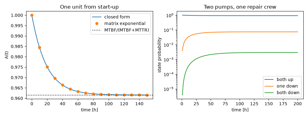
two pumps, one crew: unavailability 2.95e-03 (balance equations 2.95e-03)
improvement over one pump: 13x