Watson’s fault tree (1961)

In 1961 the US Air Force asked Bell Telephone Laboratories whether the Minuteman launch-control system could fire a missile without a valid order. H. A. Watson’s answer was a new diagram, the fault tree. It starts from the undesired top event and works downward through AND gates (every input must happen) and OR gates (any input will do) until it reaches basic failures whose probabilities are known (fault_tree_probability()). Boeing took the method into the rest of the Minuteman programme, and it spread to aviation and nuclear safety. One trap is an event that feeds more than one branch: the gate inputs are then dependent, and combining gates one by one gives the wrong answer.

import matplotlib.pyplot as plt
import numpy as np

from engineeringkit.reliability import fault_tree_probability

An illustrative launch-signal tree

A spurious launch signal needs both relays to stick, or a power-supply transient together with a failed interlock switch or an operator error. The power transient appears in two branches. Probabilities are per alert period and are invented for the illustration.

p = {"relay A": 0.02, "relay B": 0.03, "power transient": 0.1, "interlock switch": 0.05, "operator error": 0.2}
tree = (
    "or",
    ("and", "relay A", "relay B"),
    ("and", "power transient", "interlock switch"),
    ("and", "power transient", "operator error"),
)
exact = fault_tree_probability(tree, p)

# Combining the three AND gates as if they were independent.
gates = [p["relay A"] * p["relay B"], p["power transient"] * p["interlock switch"], p["power transient"] * p["operator error"]]
gate_by_gate = 1 - np.prod([1 - g for g in gates])
# The same logic with the shared event factored out has no repeats.
factored = ("or", ("and", "relay A", "relay B"), ("and", "power transient", ("or", "interlock switch", "operator error")))
rare_event = sum(gates)
print(f"exact top event {exact:.5f}; factored tree {fault_tree_probability(factored, p):.5f}")
print(f"gate by gate (wrong) {gate_by_gate:.5f}; sum of minimal cut sets {rare_event:.5f}")
assert np.isclose(exact, fault_tree_probability(factored, p))
assert gate_by_gate > exact

exact top event 0.02459; factored tree 0.02459
gate by gate (wrong) 0.02549; sum of minimal cut sets 0.02560

Check by simulation

rng = np.random.default_rng(1961)
draws = {name: rng.random(1_000_000) < q for name, q in p.items()}
top = (draws["relay A"] & draws["relay B"]) | (draws["power transient"] & (draws["interlock switch"] | draws["operator error"]))
print(f"Monte Carlo {top.mean():.5f} +/- {top.std() / np.sqrt(top.size):.5f}")
assert abs(top.mean() - exact) < 4 * top.std() / np.sqrt(top.size)

Monte Carlo 0.02444 +/- 0.00015

The error grows with the shared event’s probability

q_power = np.linspace(0.01, 0.9, 60)
exact_curve, naive_curve = [], []
for q in q_power:
    pq = {**p, "power transient": q}
    exact_curve.append(fault_tree_probability(tree, pq))
    naive_curve.append(1 - (1 - pq["relay A"] * pq["relay B"]) * (1 - q * pq["interlock switch"]) * (1 - q * pq["operator error"]))

error = 100 * (np.array(naive_curve) / np.array(exact_curve) - 1)
print(f"gate-by-gate error: {error[0]:.1f}% at q = {q_power[0]:.2f}, {error.max():.1f}% at most")
assert np.all(error > 0)

fig, axes = plt.subplots(1, 2, figsize=(10, 3.8))
axes[0].plot(q_power, exact_curve, label="exact (repeated event handled)")
axes[0].plot(q_power, naive_curve, "--", label="gate by gate, as if independent")
axes[0].set(xlabel="probability of a power transient", ylabel="top-event probability", title="Top event")
axes[0].legend(fontsize=8)
axes[1].plot(q_power, error, "C3")
axes[1].axvline(p["power transient"], color="k", ls=":", lw=1)
axes[1].set(xlabel="probability of a power transient", ylabel="overestimate [%]", title="Error of treating the gates as independent")
fig.tight_layout()

plt.show()

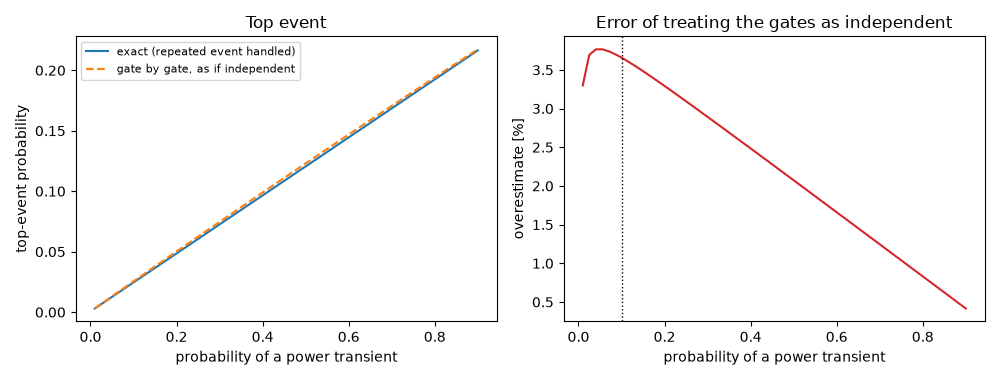
gate-by-gate error: 3.3% at q = 0.01, 3.8% at most