Metropolis and Ulam’s Monte Carlo method (1949)

Stanislaw Ulam, recovering from an illness and playing solitaire, wondered whether it was quicker to estimate the chance of winning by dealing many games than by combinatorics. With Nicholas Metropolis (1949) he described the Monte Carlo method: estimate a probability or an integral by random sampling. For a structure the failure probability \(P(g(X) < 0)\) is the fraction of sampled load and resistance pairs that fail (monte_carlo_failure_probability()). It needs no linearisation, which makes it the check on the Hasofer-Lind index (hasofer_lind_index()), but its relative error falls only as \(1/\sqrt{N p_f}\). Sampling around the Hasofer-Lind design point instead of the mean (importance sampling) puts half the samples in the failure domain.

import matplotlib.pyplot as plt
import numpy as np

from engineeringkit.reliability import hasofer_lind_index, monte_carlo_failure_probability

A nonlinear limit state

A steel tie of yield stress \(f_y\) ~ N(350, 25) MPa and area \(A\) ~ N(1000, 50) mm² carries a load \(P\) ~ N(200, 30) kN: \(g = f_y A - P\), in kN. The product makes the limit state curved, so FORM’s \(\Phi(-\beta)\) is not exact.

def g(x):
    return x[0] * x[1] / 1000 - x[2]


mean, std = [350.0, 1000.0, 200.0], [25.0, 50.0, 30.0]
form = hasofer_lind_index(g, mean, std)
reference = monte_carlo_failure_probability(g, mean, std, samples=4_000_000, seed=1949)
print(f"Hasofer-Lind beta = {form.beta:.3f}, FORM p_f = {form.failure_probability:.3e}")
print(f"Monte Carlo (4e6 samples) p_f = {reference.failure_probability:.3e} +/- {reference.std_error:.1e}")

Hasofer-Lind beta = 3.590, FORM p_f = 1.656e-04
Monte Carlo (4e6 samples) p_f = 1.735e-04 +/- 6.6e-06

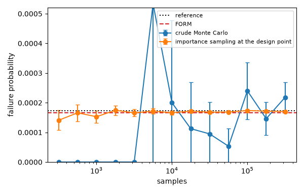
Convergence: crude sampling against importance sampling

sizes = np.logspace(2.5, 5.5, 13).astype(int)
crude = [monte_carlo_failure_probability(g, mean, std, samples=n, seed=n) for n in sizes]
weighted = [monte_carlo_failure_probability(g, mean, std, samples=n, seed=n, center=form.design_point) for n in sizes]
fig, ax = plt.subplots(figsize=(6, 3.8))
for label, runs in (("crude Monte Carlo", crude), ("importance sampling at the design point", weighted)):
    pf = np.array([run.failure_probability for run in runs])
    error = np.array([run.std_error for run in runs])
    ax.errorbar(sizes, pf, yerr=1.96 * error, fmt="o-", capsize=3, label=label)
ax.axhline(reference.failure_probability, color="k", ls=":", label="reference")
ax.axhline(form.failure_probability, color="C3", ls="--", label="FORM")
ax.set(xscale="log", xlabel="samples", ylabel="failure probability", ylim=(0, 3 * reference.failure_probability))
ax.legend(fontsize=8)
fig.tight_layout()

n = sizes[-1]
print(f"{n} samples: crude CoV {crude[-1].cov:.3f}, importance sampling CoV {weighted[-1].cov:.4f}")
print(f"samples for 10% crude accuracy: about {100 / reference.failure_probability:.0f}")

assert abs(weighted[-1].failure_probability - reference.failure_probability) < 4 * np.hypot(weighted[-1].std_error, reference.std_error)
assert weighted[-1].cov < crude[-1].cov / 10
assert reference.confidence_interval(0.999)[0] < reference.failure_probability < reference.confidence_interval(0.999)[1]

plt.show()

316227 samples: crude CoV 0.120, importance sampling CoV 0.0036
samples for 10% crude accuracy: about 576369