Hasofer and Lind’s reliability index (1974)

Cornell’s 1969 index, mean over standard deviation of the safety margin \(g\), has a flaw: it changes when the same failure condition is written differently, say \(R - S < 0\) or \(R/S - 1 < 0\). Hasofer and Lind (1974) fixed it by measuring, in standardised variables, the shortest distance from the mean to the failure surface itself (hasofer_lind_index()). The nearest point, the design point, is where failure is most likely to happen, and \(p_f \approx \Phi(-\beta)\).

import matplotlib.pyplot as plt
import numpy as np

from engineeringkit.reliability import failure_probability_from_index, hasofer_lind_index

Invariance to how the limit state is written

Resistance \(R\) ~ N(500, 50) kN, load \(S\) ~ N(300, 60) kN. Cornell’s mean-value index uses the first-order mean and standard deviation of \(g\) at the mean point.

mean, std = np.array([500.0, 300.0]), np.array([50.0, 60.0])
forms = {"R - S": lambda x: x[0] - x[1], "R/S - 1": lambda x: x[0] / x[1] - 1, "ln(R/S)": lambda x: np.log(x[0] / x[1])}
cornell, hl = {}, {}
for name, g in forms.items():
    h = 1e-6 * mean
    grad = np.array([(g(mean + h * e) - g(mean - h * e)) / (2 * h[i]) for i, e in enumerate(np.eye(2))])
    cornell[name] = g(mean) / np.linalg.norm(grad * std)
    hl[name] = hasofer_lind_index(g, mean, std)
    print(f"g = {name:8s}: Cornell beta = {cornell[name]:.3f}, Hasofer-Lind beta = {hl[name].beta:.3f}")

g = R - S   : Cornell beta = 2.561, Hasofer-Lind beta = 2.561
g = R/S - 1 : Cornell beta = 1.789, Hasofer-Lind beta = 2.561
g = ln(R/S) : Cornell beta = 2.284, Hasofer-Lind beta = 2.561

The design point and a Monte Carlo check

result = hl["R - S"]
rng = np.random.default_rng(1974)
samples = rng.normal(mean, std, size=(2_000_000, 2))
pf_mc = np.mean(samples[:, 0] < samples[:, 1])
print(f"design point R = S = {result.design_point[0]:.1f} kN; alpha^2 = {np.round(result.alpha**2, 3)}")
print(f"FORM p_f = {result.failure_probability:.2e}, Monte Carlo {pf_mc:.2e}")

fig, ax = plt.subplots(figsize=(5.5, 5))
u = np.linspace(-5, 5, 200)
U1, U2 = np.meshgrid(u, u)
G = (mean[0] + std[0] * U1) - (mean[1] + std[1] * U2)
ax.contourf(U1, U2, G < 0, levels=[0.5, 1.5], colors=["C3"], alpha=0.25)
ax.contour(U1, U2, G, levels=[0], colors="C3")
for radius in (1, 2, 3):
    ax.add_patch(plt.Circle((0, 0), radius, fill=False, ls=":", color="gray"))
u_star = (result.design_point - mean) / std
ax.plot([0, u_star[0]], [0, u_star[1]], "k-o")
ax.annotate(rf"$\beta$ = {result.beta:.2f}", u_star / 2, textcoords="offset points", xytext=(8, -4))
ax.set(xlabel="$u_R$", ylabel="$u_S$", aspect="equal", title="Standard normal space")
fig.tight_layout()

assert max(hl[k].beta for k in hl) - min(hl[k].beta for k in hl) < 1e-5
assert max(cornell.values()) - min(cornell.values()) > 0.5
assert np.isclose(result.failure_probability, pf_mc, rtol=0.05)
assert np.isclose(failure_probability_from_index(result.beta), result.failure_probability)

plt.show()

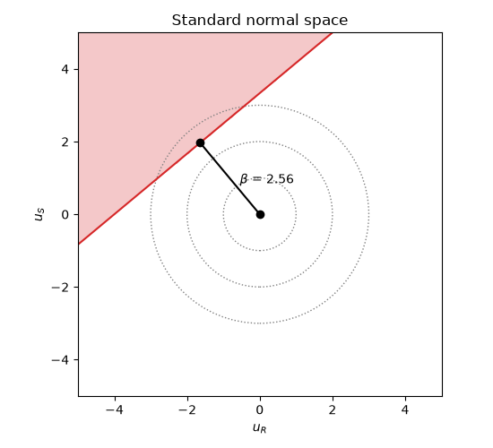
design point R = S = 418.0 kN; alpha^2 = [0.41 0.59]
FORM p_f = 5.22e-03, Monte Carlo 5.19e-03