The AGREE report: series systems and MTBF (1957)

In the early 1950s, most of the US Navy’s electronics was out of action at any given time, largely because of vacuum-tube failures. The Advisory Group on Reliability of Electronic Equipment (AGREE) reported in 1957 that reliability must be specified as a number, predicted and demonstrated by test. Its working model was a series system of parts with constant failure rates: the system’s hazard (exponential_hazard()) is the sum of the parts’ rates and its MTBF the reciprocal. More parts means less reliability, \(R_s = \prod R_i\) (series_reliability()).

import matplotlib.pyplot as plt
import numpy as np

from engineeringkit.reliability import (
    exponential_failure_probability,
    exponential_hazard,
    exponential_mttf,
    exponential_reliability,
    series_reliability,
)

A parts-count prediction

An illustrative 1950s receiver; part rates are representative, per hour.

parts = {
    "vacuum tubes": (40, 5e-5),
    "resistors": (300, 1e-7),
    "capacitors": (150, 5e-7),
    "transformers": (12, 2e-6),
    "relays": (8, 1e-5),
    "solder joints": (2000, 5e-9),
}
rates = {name: count * exponential_hazard(rate) for name, (count, rate) in parts.items()}
lam_sys = sum(rates.values())
mtbf = exponential_mttf(lam_sys)
for name, rate in sorted(rates.items(), key=lambda kv: -kv[1]):
    print(f"{name:14s} {rate:.2e}/h ({rate / lam_sys:5.1%})")
print(f"system rate {lam_sys:.2e}/h, MTBF {mtbf:.0f} h")

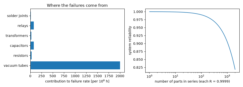
vacuum tubes   2.00e-03/h (90.1%)
relays         8.00e-05/h ( 3.6%)
capacitors     7.50e-05/h ( 3.4%)
resistors      3.00e-05/h ( 1.4%)
transformers   2.40e-05/h ( 1.1%)
solder joints  1.00e-05/h ( 0.5%)
system rate 2.22e-03/h, MTBF 451 h

The series product equals the summed-rate exponential

mission = 24.0
product = series_reliability(*[float(exponential_reliability(mission, count * rate)) for count, rate in parts.values()])
print(f"24 h mission: product of part reliabilities {product:.4f}, exp(-lambda t) {float(exponential_reliability(mission, lam_sys)):.4f}")
print(f"probability of a failure during the mission: {float(exponential_failure_probability(mission, lam_sys)):.4f}")

fig, axes = plt.subplots(1, 2, figsize=(10, 3.6))
axes[0].barh(list(rates), [rates[k] * 1e6 for k in rates])
axes[0].set(xlabel="contribution to failure rate [per $10^6$ h]", title="Where the failures come from")
n = np.arange(1, 2001)
axes[1].semilogx(n, [series_reliability(*[0.9999] * k) for k in n])
axes[1].set(xlabel="number of parts in series (each R = 0.9999)", ylabel="system reliability")
fig.tight_layout()

assert np.isclose(product, float(exponential_reliability(mission, lam_sys)))
assert np.isclose(1 - product, float(exponential_failure_probability(mission, lam_sys)))
assert max(rates, key=rates.get) == "vacuum tubes"

plt.show()

24 h mission: product of part reliabilities 0.9481, exp(-lambda t) 0.9481
probability of a failure during the mission: 0.0519