Gibbs’s phenomenon (1899)

Albert Michelson’s harmonic analyser (1898) summed 80 Fourier terms mechanically, and its curves for a square wave overshot at every jump. Michelson suspected the machine. Josiah Willard Gibbs (1899) showed in Nature that the mathematics itself overshoots: near a discontinuity the partial sums (fourier_partial_sum()) rise about 9% of the jump above it, however many terms are kept. The overshoot only narrows toward the jump. Henry Wilbraham had found the same effect in 1848, unnoticed.

import matplotlib.pyplot as plt
import numpy as np
from scipy.special import sici

from engineeringkit.signal_processing import fourier_partial_sum

A square wave and its partial sums

The square wave of period 1 and amplitude \(\pm 1\) has \(b_k = 4/(\pi k)\) for odd \(k\) and no other terms.

period = 1.0
t = np.linspace(-0.25, 0.25, 20001)
limit = 2 / np.pi * sici(np.pi)[0]  # peak of the partial sums as K grows
print(f"predicted limit of the peak: {limit:.5f} (overshoot {(limit - 1) / 2:.2%} of the jump)")

fig, axes = plt.subplots(1, 2, figsize=(10, 3.8))
peaks = {}
for K in (5, 25, 125, 625):
    k = np.arange(1, K + 1)
    b = np.where(k % 2 == 1, 4 / (np.pi * k), 0.0)
    x = fourier_partial_sum(t, period, np.zeros(K), b)
    peaks[K] = x.max()
    position = t[np.argmax(x)]
    print(f"K = {K:3d}: peak {peaks[K]:.5f} at t = {position:.5f} s")
    if K <= 125:
        axes[0].plot(t, x, lw=0.8, label=f"K = {K}")
axes[0].plot(t, np.sign(t), "k", lw=1.5, label="square wave")
axes[0].set(xlabel="t [s]", ylabel="x", title="Partial sums near the jump at t = 0")
axes[0].legend(fontsize=8)

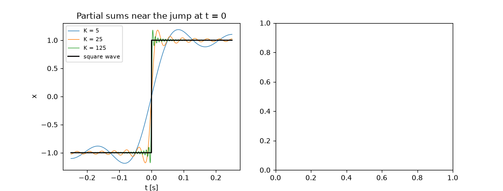
predicted limit of the peak: 1.17898 (overshoot 8.95% of the jump)
K =   5: peak 1.18836 at t = 0.08333 s
K =  25: peak 1.17947 at t = 0.01922 s
K = 125: peak 1.17900 at t = 0.00398 s
K = 625: peak 1.17898 at t = 0.00080 s

<matplotlib.legend.Legend object at 0x111108a50>

The overshoot does not shrink

The peak tends to \(\frac{2}{\pi}\operatorname{Si}(\pi) \approx 1.179\), not to 1. It sits at \(t \approx T/(2K)\), moving toward the jump.

assert abs(peaks[625] - limit) < 1e-3
assert all(p > 1.17 for p in peaks.values())

What does converge: the energy of the error

The mean squared error over a period falls like \(1/K\). Fourier series converge in energy even where they never converge uniformly.

t_period = np.linspace(-0.5, 0.5, 40001)[:-1]
Ks = np.array([5, 25, 125, 625])
mse = []
for K in Ks:
    k = np.arange(1, K + 1)
    b = np.where(k % 2 == 1, 4 / (np.pi * k), 0.0)
    mse.append(np.mean((fourier_partial_sum(t_period, period, np.zeros(K), b) - np.sign(t_period)) ** 2))
slope = np.polyfit(np.log(Ks), np.log(mse), 1)[0]
print(f"mean squared error falls as K^{slope:.2f}")
assert abs(slope + 1) < 0.1
axes[1].loglog(Ks, mse, "o-", label="mean squared error")
axes[1].loglog(Ks, np.array([peaks[K] for K in Ks]) - 1, "s-", label="overshoot")
axes[1].set(xlabel="number of terms K", title="Error energy vanishes, overshoot does not")
axes[1].legend()
fig.tight_layout()

plt.show()

mean squared error falls as K^-0.97