Cooley and Tukey’s fast Fourier transform (1965)

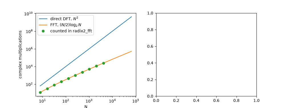
A direct DFT of \(N\) samples needs \(N^2\) complex multiplications. James Cooley and John Tukey (1965) split it into the DFTs of the even- and odd-numbered samples, combined by “butterflies” \(E_k \pm W^k O_k\), and repeated the split down to single samples (radix2_fft()). The cost falls to \((N/2)\log_2 N\). Gauss had used the same idea in 1805 to interpolate asteroid orbits. In 1965 it made spectral analysis on a computer routine, and it is what dft() (NumPy’s FFT) does.

import matplotlib.pyplot as plt
import numpy as np

from engineeringkit.signal_processing import convolution, dft, fft_frequencies, radix2_fft

The butterflies give the DFT

A direct DFT is a matrix product with \(N^2\) entries \(e^{-j2\pi kn/N}\).

rng = np.random.default_rng(1965)
x = rng.normal(size=1024) + 1j * rng.normal(size=1024)
n = np.arange(x.size)
direct = np.exp(-2j * np.pi * np.outer(n, n) / x.size) @ x
fast, count = radix2_fft(x, return_multiplications=True)
assert np.allclose(fast, direct) and np.allclose(fast, dft(x))
print(f"N = {x.size}: direct {x.size**2} multiplications, radix-2 {count}, speed-up {x.size**2 / count:.0f}x")

N = 1024: direct 1048576 multiplications, radix-2 5120, speed-up 205x

Operation counts

sizes = 2 ** np.arange(3, 17)
counts = [radix2_fft(np.zeros(size), return_multiplications=True)[1] for size in sizes[:10]]
assert counts == [size // 2 * int(np.log2(size)) for size in sizes[:10]]
fig, axes = plt.subplots(1, 2, figsize=(10, 3.8))
axes[0].loglog(sizes, sizes**2, label="direct DFT, $N^2$")
axes[0].loglog(sizes, sizes / 2 * np.log2(sizes), label=r"FFT, $(N/2)\log_2 N$")
axes[0].loglog(sizes[:10], counts, "o", label="counted in radix2_fft")
axes[0].set(xlabel="N", ylabel="complex multiplications")
axes[0].legend()

<matplotlib.legend.Legend object at 0x111046c10>

Fast convolution

The FFT turns convolution into multiplication: zero-pad both sequences to the output length, multiply their transforms, and invert. For a long filter this beats the direct sum.

signal_in = rng.normal(size=4000)
h = np.exp(-np.arange(300) / 50.0)
length = int(2 ** np.ceil(np.log2(signal_in.size + h.size - 1)))
fast_conv = np.fft.ifft(dft(np.pad(signal_in, (0, length - signal_in.size))) * dft(np.pad(h, (0, length - h.size)))).real
fast_conv = fast_conv[: signal_in.size + h.size - 1]
assert np.allclose(fast_conv, convolution(signal_in, h))
print(f"FFT convolution of {signal_in.size} by {h.size} samples matches the direct sum")

fs = 1000.0
tone = np.sin(2 * np.pi * 125 * np.arange(64) / fs)
spectrum = radix2_fft(tone)
axes[1].stem(np.fft.fftshift(fft_frequencies(64, fs)), np.fft.fftshift(abs(spectrum)), basefmt=" ")
axes[1].set(xlabel="frequency [Hz]", ylabel="|X|", title="radix2_fft of a 125 Hz tone")
assert abs(fft_frequencies(64, fs)[np.argmax(abs(spectrum[:32]))] - 125) < 1e-9
fig.tight_layout()

plt.show()

FFT convolution of 4000 by 300 samples matches the direct sum