Hilbert’s conjugate functions and the analytic signal (1905)

In his third communication on integral equations (1905), David Hilbert paired a function on the unit circle with its conjugate, the boundary values of the real and imaginary parts of one analytic function, through the singular kernel \(\cot\frac{s - t}{2}\). In frequency terms the pairing shifts every component by -90°: \(\cos \to \sin\). Dennis Gabor (1946) added the conjugate to a real signal as its imaginary part, \(z = x + j\mathcal{H}x\), and called the result the analytic signal: it has no negative frequencies, its magnitude is the envelope and its phase advances at the instantaneous frequency (hilbert_transform(), analytic_signal(), envelope(), instantaneous_frequency(), hilbert_fir()). The 1905 date and pages come from the Göttingen Nachrichten catalogue record; that the transform pair appears there follows F. W. King, Hilbert Transforms (Cambridge, 2009), a secondary source.

import matplotlib.pyplot as plt
import numpy as np

from engineeringkit.signal_processing import (
    analytic_signal,
    db20,
    envelope,
    filter_signal,
    frequency_response,
    hilbert_fir,
    hilbert_transform,
    instantaneous_frequency,
)

A -90° shift for every frequency

fs = 1000.0
t = np.arange(1000) / fs
x = np.cos(2 * np.pi * 30 * t) + 0.5 * np.cos(2 * np.pi * 70 * t + 1.0)
expected = np.sin(2 * np.pi * 30 * t) + 0.5 * np.sin(2 * np.pi * 70 * t + 1.0)
assert np.allclose(hilbert_transform(x), expected)
Z = np.fft.fft(analytic_signal(x))
print(f"negative-frequency energy fraction: {np.sum(np.abs(Z[501:]) ** 2) / np.sum(np.abs(Z) ** 2):.1e}")

negative-frequency energy fraction: 3.9e-32

Envelope and instantaneous frequency

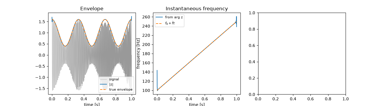
An amplitude-modulated chirp: the envelope is recovered without a rectifier and low-pass filter, and the phase slope gives the sweep.

f0, rate = 100.0, 150.0
a = 1 + 0.6 * np.cos(2 * np.pi * 3 * t)
chirp = a * np.cos(2 * np.pi * (f0 * t + rate * t**2 / 2))
env = envelope(chirp)
f_inst = instantaneous_frequency(chirp, fs)
inner = slice(100, -100)
fig, axes = plt.subplots(1, 3, figsize=(13, 3.6))
axes[0].plot(t, chirp, lw=0.5, color="0.6", label="signal")
axes[0].plot(t, env, label="|z|")
axes[0].plot(t, a, "--", label="true envelope")
axes[0].set(xlabel="time [s]", title="Envelope")
axes[0].legend(fontsize=8)
axes[1].plot(t[1:], f_inst, label="from arg z")
axes[1].plot(t, f0 + rate * t, "--", label="$f_0 + \\dot f t$")
axes[1].set(xlabel="time [s]", ylabel="frequency [Hz]", title="Instantaneous frequency")
axes[1].legend(fontsize=8)
envelope_error = np.abs(env - a)[inner].max()
frequency_error = np.abs(f_inst - (f0 + rate * (t[1:] - 0.5 / fs)))[inner].max()
print(f"envelope error {envelope_error:.3f}, frequency error {frequency_error:.2f} Hz")

envelope error 0.000, frequency error 0.03 Hz

A causal FIR Hilbert transformer

The ideal impulse response \(2/(\pi m)\) for odd \(m\) is windowed to 61 taps. Its gain is close to one away from DC and Nyquist, and its output, paired with the input delayed by 30 samples, matches the FFT-based transform.

h = hilbert_fir(61)
f, H = frequency_response(h, 1, worN=2048, fs=fs)
axes[2].plot(f, db20(np.maximum(np.abs(H), 1e-6)))
axes[2].set(xlabel="frequency [Hz]", ylabel="gain [dB]", ylim=(-20, 2), title="61-tap Hilbert FIR")
fig.tight_layout()
y = filter_signal(h, 1, x)
fir_error = np.abs(y[60:] - hilbert_transform(x)[30:-30]).max()
print(f"FIR against FFT transform: largest difference {fir_error:.3f}")
assert envelope_error < 0.02 and frequency_error < 1.0
assert fir_error < 0.02

plt.show()

FIR against FFT transform: largest difference 0.003