Ahmed, Natarajan and Rao’s discrete cosine transform (1974)

The best basis for compressing a random signal, the Karhunen-Loève transform, depends on the signal’s covariance and has no fast algorithm. Nasir Ahmed, T. Natarajan and K. R. Rao (1974) proposed a fixed basis of sampled cosines that comes very close to it for strongly correlated signals. Because the DCT implicitly extends the record by its mirror image, there is no jump at the ends and the coefficients of a smooth signal decay fast; the DFT’s periodic extension has a jump and leaks. The DCT became the core of JPEG, MPEG and MP3 (dct(), idct()).

import matplotlib.pyplot as plt
import numpy as np
from scipy import fft as sfft
from scipy import linalg

from engineeringkit.signal_processing import dct, idct

An orthonormal cosine basis

N = 16
basis = np.array([dct(row) for row in np.eye(N)]).T
assert np.allclose(basis @ basis.T, np.eye(N))
x = np.random.default_rng(1974).normal(size=N)
assert np.allclose(dct(x), sfft.dct(x, norm="ortho")) and np.allclose(idct(dct(x)), x)
fig, axes = plt.subplots(1, 3, figsize=(13, 3.6))
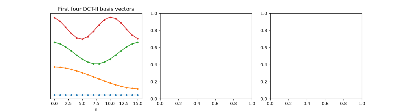
for k in range(4):
    axes[0].plot(basis[k] + 0.8 * k, "o-", ms=3)
axes[0].set(xlabel="n", yticks=[], title="First four DCT-II basis vectors")

[Text(0.5, 10.433333333333328, 'n'), [], Text(0.5, 1.0, 'First four DCT-II basis vectors')]

Close to Karhunen-Loève for a Markov process

For a first-order process with correlation \(\rho\), compare how much of the expected energy the best \(m\) coefficients of each basis hold. The KLT is the optimum; the DCT nearly matches it, the DFT does not.

rho = 0.95
R = linalg.toeplitz(rho ** np.arange(N))
klt = np.sort(np.linalg.eigvalsh(R))[::-1]
dct_var = np.sort(np.diag(basis @ R @ basis.T))[::-1]
F = np.fft.fft(np.eye(N)) / np.sqrt(N)
dft_var = np.sort(np.real(np.diag(F @ R @ F.conj().T)))[::-1]
m = np.arange(1, N + 1)
for name, variances in (("KLT", klt), ("DCT", dct_var), ("DFT", dft_var)):
    axes[1].plot(m, np.cumsum(variances) / N, "o-", ms=3, label=name)
share = {name: np.cumsum(v)[3] / N for name, v in (("KLT", klt), ("DCT", dct_var), ("DFT", dft_var))}
print({k: round(float(v), 4) for k, v in share.items()}, "of the energy in 4 of 16 coefficients")
axes[1].set(xlabel="coefficients kept", ylabel="energy fraction", title=f"Markov process, rho = {rho}")
axes[1].legend()

{'KLT': 0.9559, 'DCT': 0.9557, 'DFT': 0.9311} of the energy in 4 of 16 coefficients

<matplotlib.legend.Legend object at 0x7fa1ee656d20>

Transform coding

Store 8 real numbers for a 64-sample exponential: the 8 largest DCT coefficients, or the 4 largest complex coefficients of the real DFT. The DFT sees a jump from \(e\) back to 1 at the period boundary and rings.

t = np.linspace(0, 1, 64)
smooth = np.exp(t)
errors = {}
for name, forward, inverse, kept in (
    ("DCT", dct, idct, 8),
    ("DFT", np.fft.rfft, lambda X: np.fft.irfft(X, 64), 4),
):
    X = forward(smooth)
    X[np.argsort(np.abs(X))[:-kept]] = 0
    rebuilt = inverse(X)
    errors[name] = float(np.sqrt(np.mean((rebuilt - smooth) ** 2)))
    axes[2].plot(t, rebuilt, label=f"{name}: rms error {errors[name]:.4f}")
axes[2].plot(t, smooth, "k:", label="signal")
axes[2].set(xlabel="t", title="8 stored numbers of 64")
axes[2].legend(fontsize=8)
fig.tight_layout()
print(errors)
assert share["KLT"] - share["DCT"] < 0.01 < share["KLT"] - share["DFT"]
assert errors["DCT"] < errors["DFT"] / 10

plt.show()

{'DCT': 0.010893222395450246, 'DFT': 0.20846658127812592}