Schafer and Rabiner’s digital interpolation (1973)

Changing a sampling rate used to mean converting back to analog and sampling again. Ronald Schafer and Lawrence Rabiner (1973), at Bell Labs, showed it is a digital filtering problem. To raise the rate by \(L\), insert \(L - 1\) zeros between samples, which leaves images of the spectrum, and remove them with a low-pass filter of gain \(L\). To lower it by \(M\), low-pass filter first so nothing aliases, then keep every \(M\)-th sample (upsample(), interpolate(), downsample(), decimate()). A windowed-sinc interpolator passes the original samples through unchanged.

import matplotlib.pyplot as plt
import numpy as np

from engineeringkit.signal_processing import decimate, downsample, interpolate, upsample, windowed_spectrum

Zeros, images and the interpolating filter

Interpolate a 50 Hz tone sampled at 400 Hz by 4. Upsampling alone puts images at 350, 450 and 750 Hz; the filter removes them.

fs, L = 400.0, 4
n = np.arange(400)
x = np.sin(2 * np.pi * 50 * n / fs)
u = upsample(x, L)
y = interpolate(x, L)
fig, axes = plt.subplots(1, 3, figsize=(13, 3.6))
for signal_, label in ((u, "upsampled (zeros)"), (y, "interpolated")):
    f, magnitude = windowed_spectrum(signal_, L * fs)
    axes[0].plot(f, 20 * np.log10(np.maximum(magnitude / magnitude.max(), 1e-6)), label=label)
    if signal_ is y:
        image = 20 * np.log10(magnitude[np.argmin(np.abs(f - 350))] / magnitude.max())
axes[0].set(xlabel="frequency [Hz]", ylabel="level [dB]", ylim=(-110, 5), title=f"Rate x{L}")
axes[0].legend(fontsize=8)
print(f"image at 350 Hz after interpolation: {image:.0f} dB")
t_fine = np.arange(y.size) / (L * fs)
axes[1].plot(t_fine[160:200], y[160:200], ".-", label="interpolated")
axes[1].plot(t_fine[160:200:L], x[40:50], "o", mfc="none", ms=8, label="original samples")
axes[1].set(xlabel="time [s]", title="Original samples pass through")
axes[1].legend(fontsize=8)
inner = slice(200, -200)
fine_error = np.abs(y - np.sin(2 * np.pi * 50 * t_fine))[inner].max()
print(f"largest error against the true tone at 1.6 kHz: {fine_error:.1e}")

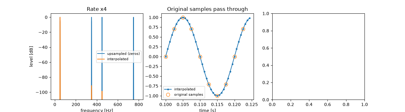
image at 350 Hz after interpolation: -91 dB
largest error against the true tone at 1.6 kHz: 4.2e-05

Decimation needs its filter

At 1 kHz, a 30 Hz tone plus a 230 Hz interferer. Keeping every 4th sample folds 230 Hz onto 20 Hz; decimating removes it first.

fs2, M = 1000.0, 4
m = np.arange(4000)
wanted = np.sin(2 * np.pi * 30 * m / fs2)
mixed = wanted + 0.5 * np.sin(2 * np.pi * 230 * m / fs2)
reference = downsample(wanted, M)
for record, label in ((downsample(mixed, M), "downsample only"), (decimate(mixed, M), "decimate")):
    f, magnitude = windowed_spectrum(record, fs2 / M)
    axes[2].plot(f, 20 * np.log10(np.maximum(magnitude / magnitude.max(), 1e-6)), label=label)
axes[2].set(xlabel="frequency [Hz]", ylabel="level [dB]", ylim=(-100, 5), title="Rate /4: 230 Hz aliases to 20 Hz")
axes[2].legend(fontsize=8)
fig.tight_layout()
alias_error = np.abs(downsample(mixed, M) - reference)[50:-50].max()
decimated_error = np.abs(decimate(mixed, M) - reference)[50:-50].max()
print(f"error against the clean tone: downsampled {alias_error:.2f}, decimated {decimated_error:.4f}")
assert np.allclose(y[::L], x)
assert image < -50 and fine_error < 0.01
assert alias_error > 0.4 > 0.01 > decimated_error

plt.show()

error against the clean tone: downsampled 0.50, decimated 0.0011