Shannon’s sampling theorem and aliasing (1949)

Claude Shannon’s 1949 paper Communication in the presence of noise opens with a theorem: a signal with no frequencies above \(B\) is completely determined by samples taken every \(1/(2B)\) seconds. Whittaker (1915), Nyquist (1928) and Kotelnikov (1933) had come close, but Shannon stated it plainly and gave the reconstruction, a sum of sinc pulses centred on the samples (sinc_reconstruct()). A frequency above the Nyquist frequency \(f_s/2\) (nyquist_frequency()) produces exactly the same samples as one below it, its alias (alias_frequency()), and no processing after the sampler can tell them apart.

import matplotlib.pyplot as plt
import numpy as np

from engineeringkit.signal_processing import alias_frequency, nyquist_frequency, sampling_period, sinc_reconstruct

Reconstruction from samples

Two tones below the Nyquist frequency, sampled at 100 Hz for 2 s. Away from the ends of the record, where the truncated sinc sum is missing terms, the reconstruction matches the signal between the samples.

fs = 100.0
T = sampling_period(fs)
n = np.arange(200)


def x_true(t):
    return np.sin(2 * np.pi * 7 * t) + 0.5 * np.cos(2 * np.pi * 31 * t)


t = np.linspace(0, 2, 4001)
rebuilt = sinc_reconstruct(x_true(n * T), fs, t)
middle = (t > 0.5) & (t < 1.5)
error = np.abs(rebuilt - x_true(t))[middle].max()
print(f"T = {T * 1e3:.0f} ms, Nyquist frequency {nyquist_frequency(fs):.0f} Hz; largest mid-record error {error:.3f}")
assert np.allclose(sinc_reconstruct(x_true(n * T), fs, n * T), x_true(n * T))
assert error < 0.05

T = 10 ms, Nyquist frequency 50 Hz; largest mid-record error 0.001

Aliasing

A 70 Hz tone sampled at 100 Hz gives the same samples as a 30 Hz tone, and the reconstruction returns the 30 Hz one.

f_high = 70.0
f_alias = alias_frequency(f_high, fs)
print(f"{f_high:.0f} Hz sampled at {fs:.0f} Hz appears at {f_alias:.0f} Hz")
assert f_alias == 30.0
assert np.allclose(np.cos(2 * np.pi * f_high * n * T), np.cos(2 * np.pi * f_alias * n * T))
wrong = sinc_reconstruct(np.cos(2 * np.pi * f_high * n * T), fs, t)
assert np.abs(wrong - np.cos(2 * np.pi * f_alias * t))[middle].max() < 0.05

fig, axes = plt.subplots(1, 3, figsize=(12, 3.6))
zoom = (t > 0.9) & (t < 1.1)
axes[0].plot(t[zoom], x_true(t[zoom]), "k", lw=2, label="signal")
axes[0].plot(t[zoom], rebuilt[zoom], "C1--", label="sinc reconstruction")
in_zoom = (n * T > 0.9) & (n * T < 1.1)
axes[0].plot((n * T)[in_zoom], x_true(n * T)[in_zoom], "o", label="samples")
axes[0].set(xlabel="time [s]", title="Below Nyquist: recovered")
axes[0].legend(fontsize=8)
axes[1].plot(t[zoom], np.cos(2 * np.pi * f_high * t[zoom]), "k", lw=1, label="70 Hz")
axes[1].plot(t[zoom], wrong[zoom], "C3", label="reconstruction (30 Hz)")
axes[1].plot((n * T)[in_zoom], np.cos(2 * np.pi * f_high * n * T)[in_zoom], "o")
axes[1].set(xlabel="time [s]", title="Above Nyquist: aliased")
axes[1].legend(fontsize=8)
f = np.linspace(0, 300, 601)
axes[2].plot(f, alias_frequency(f, fs))
axes[2].set(xlabel="input frequency [Hz]", ylabel="apparent frequency [Hz]", title="Folding about fs/2")
fig.tight_layout()

plt.show()

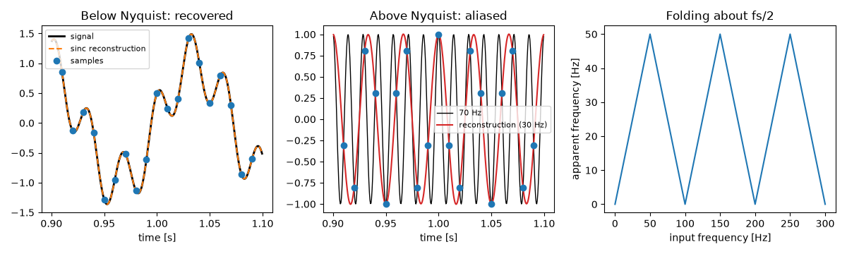
70 Hz sampled at 100 Hz appears at 30 Hz