Schuster’s periodogram (1898)

Was there a 26-day period in the weather, linked to the Sun’s rotation? Arthur Schuster (1898) answered such questions with the periodogram: the squared magnitude of the record’s Fourier coefficients, \(|X_k|^2/N\), plotted against period (dft(), power_spectral_density()). A true periodicity stands out as a peak that grows with the record length, while the noise level does not. Schuster also worked out how high a peak pure noise is likely to throw up. The example hides a weak sine in noise several times stronger and finds it.

import matplotlib.pyplot as plt
import numpy as np

from engineeringkit.signal_processing import Spectrum, dft, energy, idft, power_spectral_density

A weak periodicity in daily data

Three years of daily values: a 26-day sine of amplitude 0.5 buried in Gaussian noise of standard deviation 2, a signal-to-noise ratio of -12 dB. The cycle cannot be seen in the record itself.

rng = np.random.default_rng(1898)
fs = 1.0  # samples per day
days = np.arange(3 * 365)
x = 0.5 * np.sin(2 * np.pi * days / 26) + rng.normal(0, 2, days.size)
frequency, psd = power_spectral_density(x, fs)
peak = frequency[1:][np.argmax(psd[1:])]
print(f"periodogram peak at a period of {1 / peak:.1f} days")
assert abs(1 / peak - 26) < 0.5

periodogram peak at a period of 26.1 days

The DFT keeps all the information

The periodogram is built on the DFT, which is invertible and, by Parseval’s theorem, preserves energy: \(\sum |x_n|^2 = \frac1N\sum |X_k|^2\). Spectrum gives the same one-sided magnitudes.

X = dft(x)
assert np.allclose(idft(X).real, x)
assert np.isclose(energy(x), energy(X) / x.size)
spectrum = Spectrum.from_signal(x - x.mean(), fs)
assert np.allclose(2 * spectrum.magnitude[1:] ** 2 / (fs * x.size), psd[1:])
print("Spectrum summary:", spectrum.summary())

Spectrum summary: {'bins': 548, 'resolution': 0.0009132420091324201, 'peak_frequency': 0.038356164383561646}

Longer records make the peak taller, not the noise smoother

The sine’s peak grows in proportion to the record length while the noise periodogram stays at \(2\sigma^2/f_s\) on average. That is why Schuster could find a weak cycle given enough data, and also why the noise itself never averages out (see Welch’s method).

fig, axes = plt.subplots(1, 2, figsize=(10, 3.8))
heights = []
for years in (1, 3, 9):
    n = years * 365
    t = np.arange(n)
    record = 0.5 * np.sin(2 * np.pi * t / 26) + rng.normal(0, 2, n)
    f, p = power_spectral_density(record, fs)
    heights.append(p[np.argmin(abs(f - 1 / 26))])
    axes[0].plot(f, p, lw=0.7, label=f"{years} yr")
    noise_level = np.median(p[f > 0.1])
    print(f"{years} yr: peak {heights[-1]:7.1f}, median noise level {noise_level:5.1f} (2 sigma^2 ln 2 = {8 * np.log(2):.1f})")
assert heights[0] < heights[1] < heights[2]
axes[0].set(xlabel="frequency [1/day]", ylabel="PSD [units$^2$ day]", xlim=(0, 0.1))
axes[0].legend()
axes[1].plot(days[:200], x[:200], lw=0.7)
axes[1].plot(days[:200], 0.5 * np.sin(2 * np.pi * days[:200] / 26), lw=2, label="hidden 26-day cycle")
axes[1].set(xlabel="day", ylabel="value")
axes[1].legend()
fig.tight_layout()

plt.show()

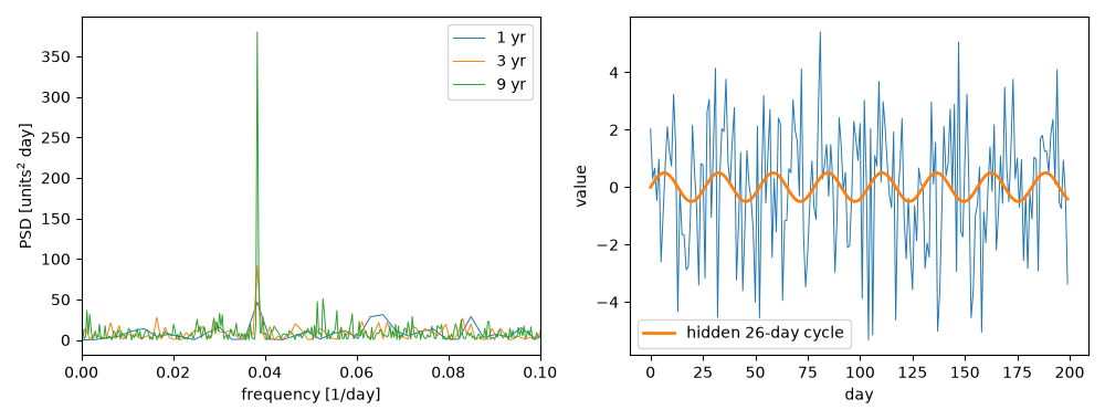
1 yr: peak    46.7, median noise level   5.9 (2 sigma^2 ln 2 = 5.5)
3 yr: peak    91.7, median noise level   5.5 (2 sigma^2 ln 2 = 5.5)
9 yr: peak   380.0, median noise level   5.4 (2 sigma^2 ln 2 = 5.5)