The Wiener-Khinchin theorem (1934)

Norbert Wiener (1930) and Aleksandr Khinchin (1934) showed that the power spectrum of a stationary random process is the Fourier transform of its autocorrelation function. A random signal has no Fourier transform of its own, but its correlation does, and that gives its spectrum a precise meaning. For a finite record the discrete version is exact: the DFT of the biased sample autocorrelation equals the periodogram (correlation(), power_spectral_density()).

import matplotlib.pyplot as plt
import numpy as np

from engineeringkit.signal_processing import correlation, dft, filter_signal, power_spectral_density

An exact identity for a finite record

correlation(x, x) returns lags \(-(N-1)\) to \(N-1\). Rotating lag zero to the front and taking a DFT of length \(2N-1\) gives \(|X|^2\), the squared DFT of x zero-padded to the same length.

rng = np.random.default_rng(1934)
x = rng.normal(size=256)
n = x.size
r = correlation(x, x) / n  # biased autocorrelation estimate
from_correlation = dft(np.roll(r, -(n - 1))).real
from_signal = abs(dft(np.concatenate([x, np.zeros(n - 1)]))) ** 2 / n
print(f"largest difference: {np.max(abs(from_correlation - from_signal)):.2e}")
assert np.allclose(from_correlation, from_signal)

largest difference: 3.11e-15

A coloured process: theory against estimate

White noise through \(y_n = a y_{n-1} + e_n\) (an AR(1) process) has autocorrelation \(r_k = \sigma^2 a^{|k|}/(1-a^2)\), whose transform is the spectrum \(S(f) = \sigma^2/|1 - a e^{-j2\pi f/f_s}|^2\) per unit of \(f_s\). The sample autocorrelation of a long record follows \(a^{|k|}\), and its transform follows \(S(f)\).

a, fs = 0.8, 1.0
y = filter_signal([1.0], [1.0, -a], rng.normal(size=2**16))
lags = np.arange(-30, 31)
r_y = correlation(y, y)[y.size - 1 + lags] / y.size
r_theory = a ** abs(lags) / (1 - a**2)
assert np.allclose(r_y, r_theory, atol=0.1)

f, psd = power_spectral_density(y, fs)
theory = 2 / (fs * abs(1 - a * np.exp(-2j * np.pi * f / fs)) ** 2)  # one-sided
smoothed = np.convolve(psd, np.ones(1024) / 1024, "same")
band = (f > 0.05) & (f < 0.45)
ratio = smoothed[band] / theory[band]
print(f"smoothed periodogram / theory over the band: {ratio.min():.3f} to {ratio.max():.3f}")
assert np.all(abs(ratio - 1) < 0.15)

fig, axes = plt.subplots(1, 2, figsize=(10, 3.8))
axes[0].stem(lags, r_y, basefmt=" ", label="sample")
axes[0].plot(lags, r_theory, "r", label=r"$a^{|k|}/(1-a^2)$")
axes[0].set(xlabel="lag $k$", ylabel="autocorrelation", title="Correlation")
axes[0].legend()
axes[1].semilogy(f, psd, lw=0.3, color="0.7", label="periodogram")
axes[1].semilogy(f, smoothed, label="smoothed")
axes[1].semilogy(f, theory, "r--", label="transform of $r_k$")
axes[1].set(xlabel="frequency [cycles/sample]", ylabel="PSD", title="Spectrum")
axes[1].legend()
fig.tight_layout()

plt.show()

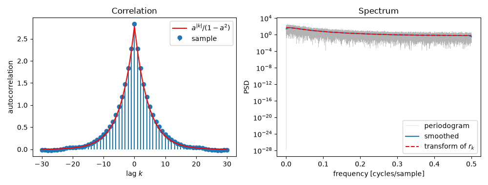
smoothed periodogram / theory over the band: 0.922 to 1.096